
Introduction
Coral reefs, although they cover less than 1% of the Earth’s surface and 2% of the seabed, support at least 25% of marine biodiversity (Spalding et al., 2001). They provide essential benefits to humanity, including maintaining the health of coastal ecosystems by facilitating important activities such as grazing, breeding, and spawning (Moberg & Folke, 1999), coastal protection (Ferrario et al., 2014), support for sustainable fisheries (Darling & D’agata, 2017), and contributions to marine tourism (Spalding et al., 2017). Additionally, coral reefs offer medicinal compounds (Cooper et al., 2014) and serve as natural laboratories for education and conservation sites (ICRI, 2020). In Indonesia, coral reefs hold significant economic value, supporting millions of communities across numerous small islands and coastal regions.
However, coral reefs are among the most vulnerable ecosystems. Nearly 20% of the world’s coral reefs are in severe decline, with estimates suggesting that 30% could experience massive damage by 2032, and many may be lost by 2050 (Hughes et al., 2017). Meanwhile, the coral reef in Indonesia ranks first globally with 18% of the world’s coral reefs, covering approximately 51,000 km², primarily located in the coral triangle, the heart of the coral reefs of the world, which boasts 83 genera and 569 species of coral (Hoeksema, 2007). However, many reefs face degradation due to declines in environmental quality (Burke et al., 2012; Pandolfi et al., 2003). In Indonesia, a study by Suharsono (unpublished; see Slide 1 coraltriangleinitiative.org) revealed that out of 1,064 observation sites, 35.2% were in poor condition (live coral cover [LCC] < 25%), 35.1% were in fair condition (LCC 25 –< 50%), 23.4% were in good condition (LCC 50 –< 75%), and only 6.4% were in excellent condition (LCC > 75%). Wulandari et al. (2022) also found poor coral health in the Selayar Biosphere Reserve at Taka Bonerate Islands.
The deterioration of coral reefs, on a local scale, is caused by various anthropogenic stressors. These include overfishing and destructive fishing practices (Jackson et al., 2001), the impact of land-based pollution such as nutrient runoff, sedimentation, and plastic pollution (Fabricius, 2005; Syakti et al., 2019), biological factors like predator population blooms of Acanthaster planci and Drupella spp snails (Brodie & McElroy, 2015; Kiel & Klemens, 2006), and coral diseases also play a significant role (Sutherland et al., 2004). On a global scale, climate change has led to ocean acidification and rising sea temperatures globally, causing coral bleaching (Hoegh-Guldberg et al., 2007; Hughes et al., 2017; Wouthuyzen et al., 2018). Those factors collectively contribute to the decline of coral reef ecosystems.
Coral reefs can recover from damage, but recovery times vary. Some species may heal in just 4 to 5 years, like those in the Marine Recreation Park of Pieh Island of west Sumatra (Wouthuyzen et al., 2019), while others may take up to 16 years (Fox et al., 2019). Therefore, mapping, monitoring, and evaluating coral reef conditions using remotely sensed satellite data is inevitable.
Various Earth observation satellites with high-resolution multispectral sensors, but those are must be purchased such as IKONOS (4 m), GeoEye-1 (1.65 m), Quickbird (1.61 m), WorldView-3 (1.24 m), and Pléiades Neo (30 cm), along with free medium-resolution options like Landsat-8/9 (30 m) and Sentinel-2 (10 m), are available for effective remote sensing. For instance, Nurdin et al. (2015) mapped coral reefs and their damages caused by destructive fishing practices using multi-temporal and multi-sensor Landsat satellite imagery in the Spermonde Islands, South Sulawesi, Indonesia, by applying image processing procedures similar to this study. Meanwhile, Aulia et al. (2020) mapped the changes of bottom benthic profile of the shallow-water coral reefs in Karya, Semak Daun Islands, and Balik Layar Reef in Seribu Islands, Indonesia, in 2016 and 2018 based on Landsat 8 (OLI) satellite imagery, which also used the same procedures as this study.
Coral reef mapping in Indonesia has utilized medium-resolution satellite data. Notable studies include Adji (2014), who mapped reefs in the Wakatobi Islands using Landsat-7. Haya & Fujii (2017) focused on the Spermonde Islands with multi-temporal Landsat data. Kartikasari et al. (2021) mapped reefs in Lovina, northern Bali, using Sentinel-2 data. However, detailed information on coral reefs in Kadatua, Liwutonkidi, and Siompu Islands in South Buton Regency, which are crucial for local livelihoods dependent on fisheries and tourism, remains lacking. The Indonesian Ministry of Marine Affairs reported 471 cases of coral damage from harmful fishing practices in South and Southeast Sulawesi from 2013 to 2019, with Kadatua, Liwutonkidi and, and Siompu Island among the affected. This study aims to map the coral reef and develop the coral reef health at five sites in these islands, aiding local coral reef management and contributing to the World Coral Reef Status Database 2025 by the Global Coral Reef Monitoring Network (GCRMN).
Material And Methods
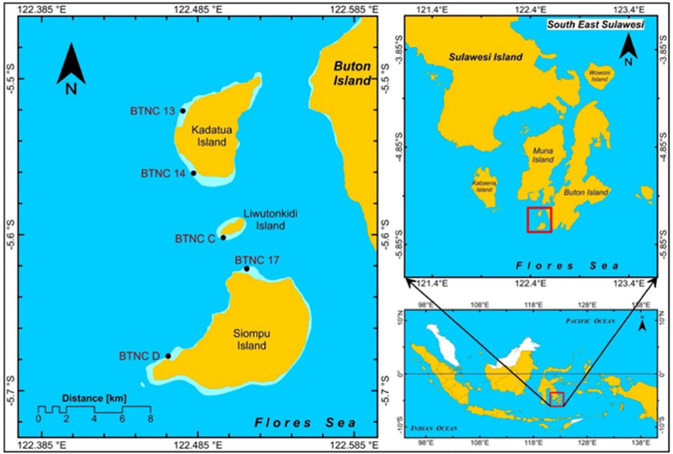
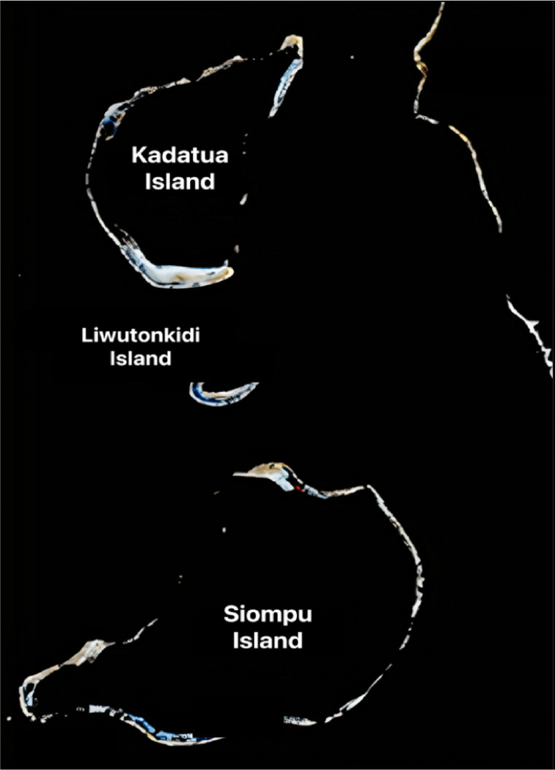
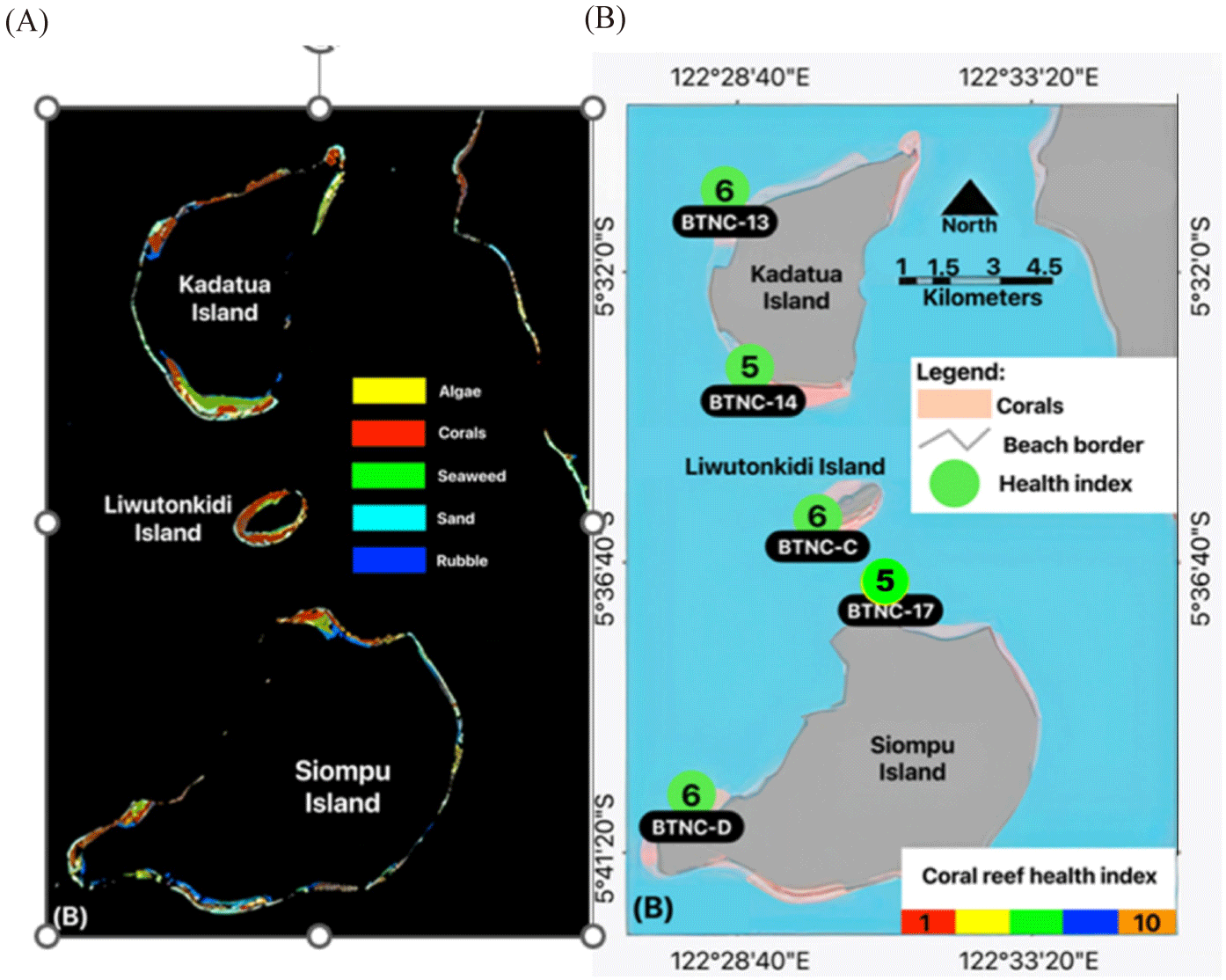
This study was conducted on Kadatua, Liwutonkidi, and Siompu Islands in South Buton Regency, Southeast Sulawesi, Indonesia, located between latitudes -5.5° to -5.7° South and longitudes 122.385 to 122.585° East. Field surveys were carried out at five locations: two on Kadatua Island (BTNC 13, BTNC 14), one on Liwutonkidi Island (BTNC C), and two on Siompu Island (BTNC 17, BTNC D), as shown in Fig. 1.
The study utilized Landsat-8 OLI satellite imagery (Path 122, Row 064) acquired in January 13, 2021. Data wa, obtained from the USGS website at https://earthexplorer.usgs.gov/. Data collection involved SCUBA diving gear, a handheld Garmin GPS, an underwater camera, and a diving slate with waterproof paper and pencils. Data processing was done using QGIS, a free and open-source GIS software.
Satellite data analysis procedures involve assessing coral reef habitat coverage and evaluating the coral reef resilience and health. The process includes two stages: pre-image and image processing. During pre-image processing, steps such as atmospheric correction, image cropping, de-glint (sun glint correction), and masking clouds and land are performed to enhance image quality (Fig. 2).
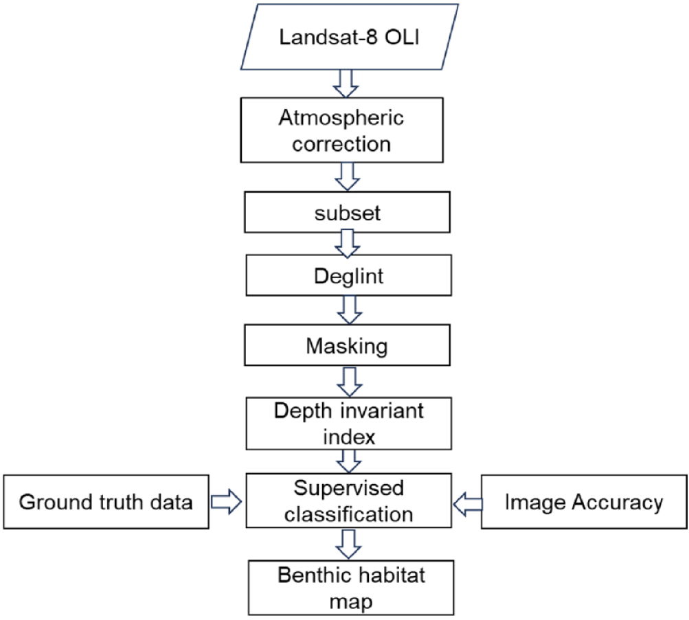
The radiometric data from Landsat-8 OLI images were corrected using the supplied metadata by converting Digital Number (DN) values into radiance or reflectance. Atmospheric influences were adjusted using the Dark Object Subtraction (DOS) method (Song et al., 2001), and the images were cropped to match the specific study sites.
To improve Landsat data quality, a sun glint correction, also known as de-glint, was applied by selecting representative pixels for different sun glint visibility levels in bands 2, 3, 4, and 5 (blue, green, red, and near-infrared [NIR]). This de-glint process follows Hedley et al. (2005) as described in Equation (1).
where: Bcorrected = de-glint corrected visible band blue, green, or red of Band-2, -3, and -4, respectively.
Bi = Landsat 8 OLI’s Visible Band 2, 3 and 4;
a and b are the intercept and slope of the regression line, respectively.
After the de-glint process, we mask the study object to isolate it from unrelated features like clouds and land. This is followed by water column correction and supervised classification using maximum likelihood (MLH) classification. The depth invariant index (DII), based on Lyzenga (1981), employs a green-red (B2-B3) band combination from the Landsat 8 OLI image to capture underwater details accurately. This correction ensures precise information about underwater objects follows the methods outlined by Green et al. (2000) and Lyzenga (1981) using the equation;
where DII is the depth Invariant Index,
Li is the digital value in band i, Lj is the digital value in band j,
Ki/kj: is the ratio of the attenuation coefficient in the band pairs i and j,
Vari: is variant band i; Varj: is variant band j; Covarij: is covariant band ij.
The attenuation coefficient is calculated by defining a region of interest (ROI) in a homogeneous area, with measurements taken at various depths. The ROI is identified through visual interpretation and underwater photography. After correcting for the water column, image classification is performed using MLH classification, which categorizes pixels based on their probability of belonging to specific classes. A pixel is not classified if its value falls below a defined threshold. Ground truthing at each data site was conducted at 62 sites using a Garmin GPS device, following SNI 7716-2011 guidelines for mapping demersal habitats in shallow waters (LIPI, 2014). Accuracy testing was done with a confusion matrix comparing classification results to field data (Congalton & Green, 2019).
To collect benthic habitat data on coral reefs, underwater photos were taken using the Photo Transect method (Giyanto & Soedarma, 2010). Observers equipped with SQUBA diving gear, underwater cameras, and bright yellow rectangular frames (58 × 44 cm) took pictures positioned 60 cm above the substrate along a 50-meter transect line (Fig. 3A). A total of 50 photos, 25 from the left and 25 from the right side along the transect line were taken.
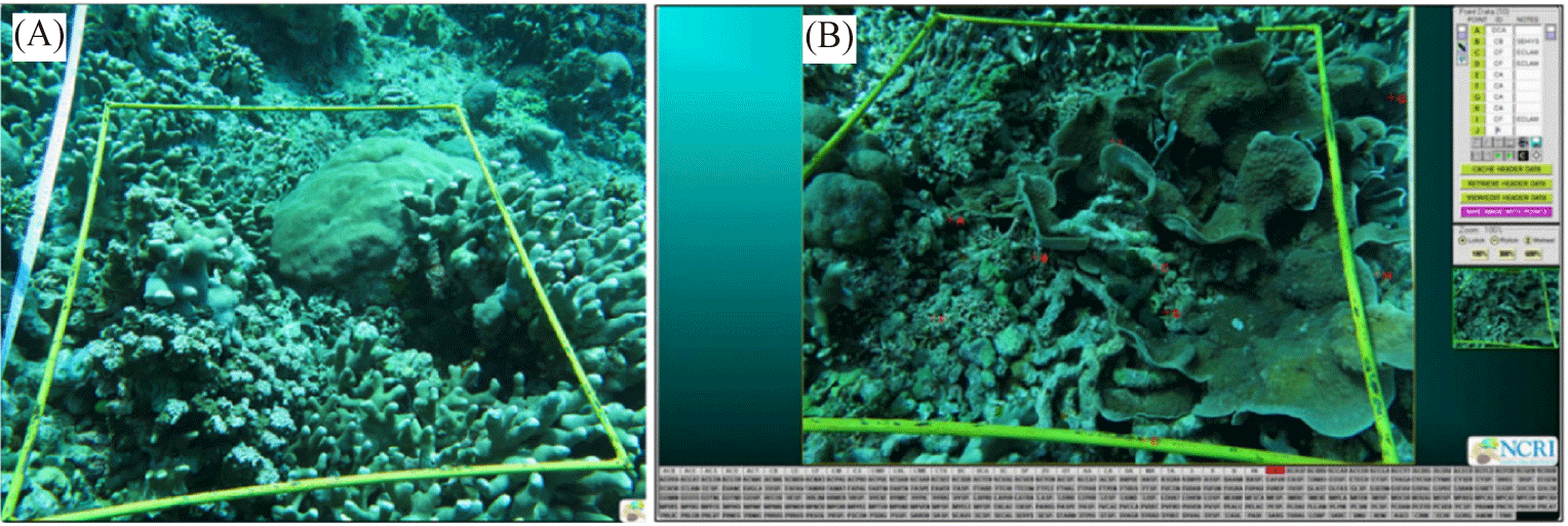
The analysis of fifty underwater photos (Fig. 3B) utilized Coral Point Count with Excel extensions (CPCe®), developed by Nova Southeastern University (Kohler & Gill, 2006). We applied a benthic component coverage technique by randomly selecting 25 points per photo and categorizing them using the CPCe® database. After exporting the results to Microsoft Excel, we calculated the percentage coverage of benthic components to assess the CHI.
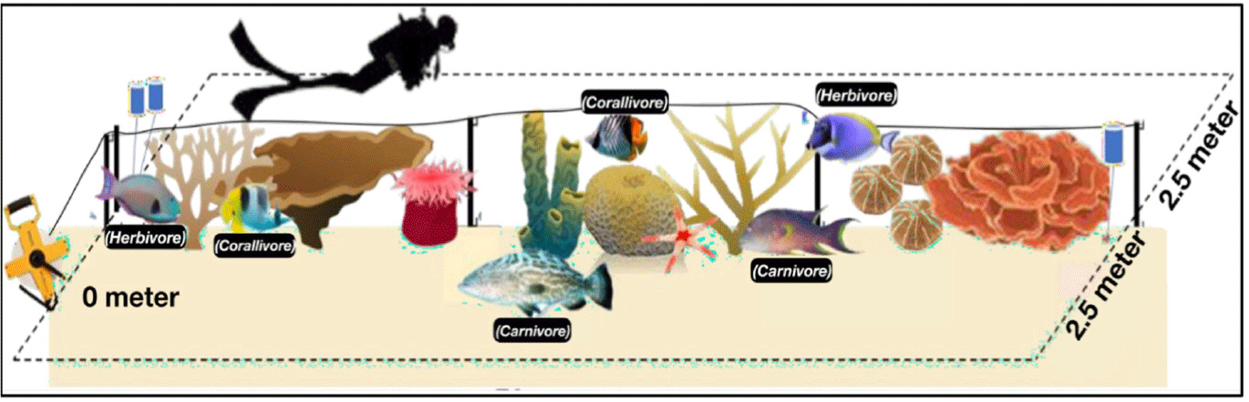
Coral reef fish observations were conducted using the underwater visual census (UVC) method from the ASEAN-Australia Project, which allows for rapid estimates of fish abundance, biomass, and distribution (Rolim et al., 2022). This assessment helps evaluate coral reef health. The UVC involved a 70-meter transect line with a 2.5-meter observation area on each side, thus resulting in a total area of 350 m² per transect, as shown in Fig. 4. The standing stock (S) of each reef fish group was calculated using the following equation:
Coral health index (CHI) is assessed based on the biomass density of reef fish, categorized into two groups: (1) Carnivorous fish (Families: Haemulidae, Lethrinidae, Lutjanidae, Serranidae), and (2) Herbivorous fish (Families: Acanthuridae, Scaridae, Siganidae). Thus, CHI was evaluated by converting the fish counts (numbers) of those groups into biomass density (B: kg/ha) using the equation:
where, S = Fish Number of a certain species;
W = a L b, W: is Weight of a certain fish species (gram or kg),
L = TL: is the total length of the fish (cm), TL=(Lmin+Lmax)/2 or TL=0.65 × Lmax, whereas Lmin and Lmax are the minimum and maximum fish TL. that can be obtained from Froese & Pauly (2018);
a and b: is the fish growth coefficient that can be cited from Kulbicki et al. (2005).
The CHI comprises several fundamental components, including the percentage of LCC, fleshy seaweed (FS) cover as indicator of recovery potential or resilience levels, and coral reef fish biomass (RFB) (Giyanto et al., 2017). The specific criteria for evaluating the coral reef's health of these components are detailed in Table 1. Meanwhile, the CHI is assessed using those components, resulting in 18 combinations of CHI values that range from 10 to 1 as detailed in Table 2. An index level of 10 in Table 2 indicates the healthiest coral reefs, characterized by high coral cover and resilience, which supports diverse coral fish and higher fish biomass. Conversely, an index value of 1 signifies poor coral cover and low resilience, hindering coral recovery and growth and correlating with very low fish biomass due to the degraded ecosystem that cannot sustain coral fish.
Data from Giyanto et al., (2017).
Data from Giyanto et al., (2017).
Results
The Landsat-8 OLI satellite image data was pre-processed to enhance clarity and minimize atmospheric interference. This interference can cause the minimum DN value for the darkest objects, such as cloud shadows and deep sea, to be zero (0). Table 3 shows a minimum DN value of 0 after atmospheric correction using the DOS method, with maximum values in most bands exceeding 100, which often occur due to a few pixels affected by thick clouds. This correction is essential for reducing atmospheric interference. Landsat-8 has 11 bands, with 30 m resolution for multispectral bands (1–7) and 15 m for the panchromatic band. In this study, we analyzed four visible bands: the Blue (Band 2), Green (Band 3), Red (Band 4), and near-infrared/NIR (Band 5) (Table 3).
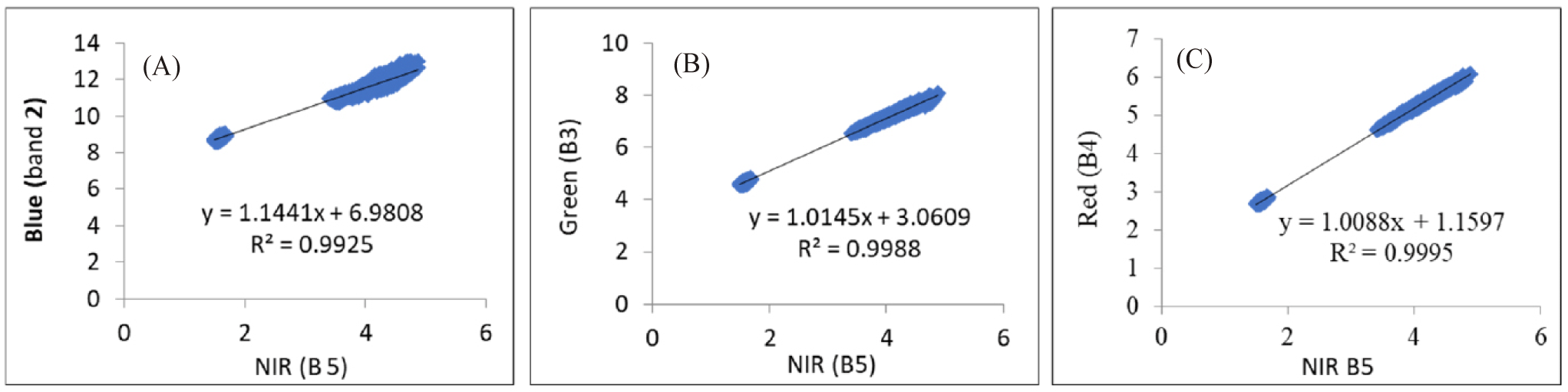
Coral reefs, seagrass, and algae habitats are often below the sea surface, making accurate identification from satellite imagery challenging due to atmospheric interference and water column effects (Chen et al., 2021). Sunlight reflection and ripples can blur these features, necessitating the correction of sun glint (Fell, 2022). In this study, sun glint was corrected using a linear regression equation that relates the Blue, Green, and Red bands to the NIR band (Hedley et al., 2005). Fig. 5 illustrates the relationship between the Blue, Green, and Red bands to the NIR bands. The minimum NIR value (NIRmin) extracted from the NIR band (Band 5) was 1.4918. The regression equation, such as that given by Equation (1) (Bi corrected = Bi – bi × [NIR − NIRmin]), is shown in Table 4. This corrected image was then used for water column attenuation correction.
Water column correction is generally used to eliminate the fading effect on an object’s signal as it travels through the water column caused by the attenuation of electromagnetic waves (Lyzenga, 1981). This attenuation leads to varying pixel values for the same object at different depths, with reflectance values decreasing as depth increases (Green et al., 2000). Thus, the correction for each band is determined using a linear regression equation based on combined visible light bands, where the slope represents the attenuation coefficient ratio (Lyzenga, 1981). Sand is chosen for sampling because it is easily identifiable at various depths; the plots of band pairs of Band 2 versus Band 3, Band 2 versus Band 4, and Band 3 versus Band 4 are shown in Fig. 6.
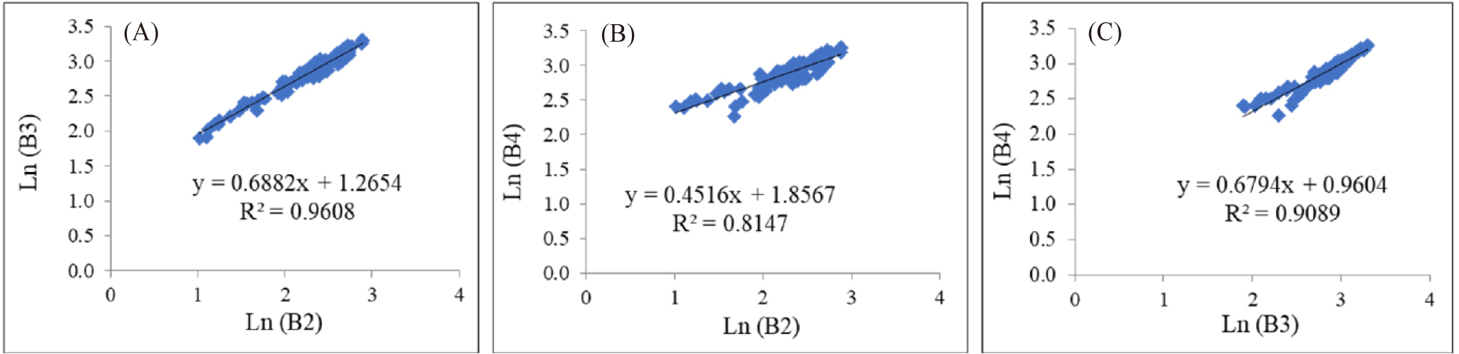
The determination coefficients (R²) of Fig. 6A–6C are considered sufficiently high to warrant further analysis. The R² values for the Band pairs of Ln(B2) vs Ln(B3) = 0.9608; Ln(B2) vs. Ln(B4) = 0.8147; and Ln(B3) vs. Ln(B4) = 0.9089. Based on the processed data at the sand area at different depths, as illustrated in Fig. 6, and the use of Equations 4, 3, and 2, the variance, covariance, parameter ‘a’, and attenuation coefficient ratios values, and DII equations can be derived as presented in Table 5 below.
Before creating the coral reef map using maximum livelihood classification, the next step after correcting the water column is masking. This process defines the boundaries of different objects in the image, such as separating the water body from the land to focus on the coral reef areas. In Fig. 7, the masking image shows that only the coral reefs have a digital reflectance value greater than zero, while the deep sea and land have zero values.
As the final stage of image processing, image classification consists of unsupervised and supervised classification (Fig. 8). The unsupervised classification was carried out to sort the visual appearance of objects based on color hues into several classes on the water column-masked image. The iterative self-organizing for the unsupervised classification technique produces eight class groups (Fig. 8A), which can be used as a tentative map for field testing using 62 ground truth points. This image was then used as the input data to classify the habitat class in the water column corrected image (Fig. 7), and the output is a distribution map of five different habitat classes, algae, corals, seaweed, sand, and rubble (Fig. 8B).
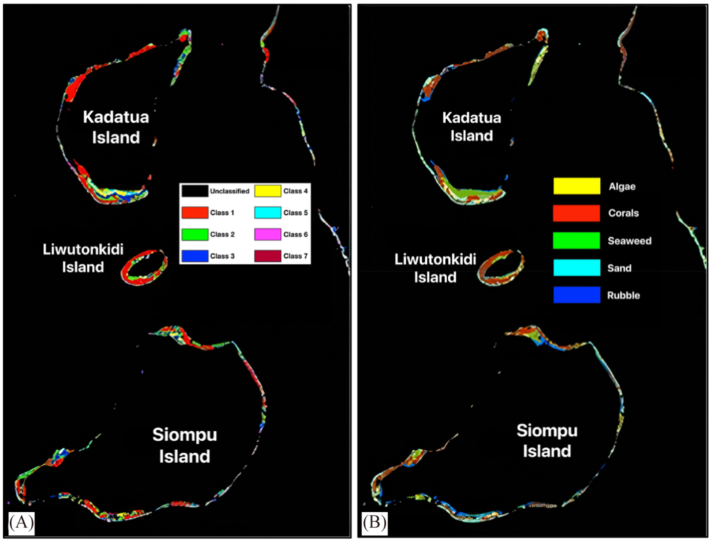
Table 6 presents the results of simple calculations assessing the accuracy of five habitat classes based on data from 62 field checkpoints (ground truth). Meanwhile, Fig. 9 illustrates the accuracy test results using a confusion matrix calculation. The findings from the simple accuracy test of Table 6 indicate an overall accuracy of 82.1%. The coral, seaweed, and sand classes have an accuracy of over 90%, with the coral class achieving the highest accuracy at 94.4%. In contrast, the algae and rubble classes display accuracies ranging from 62.5% to 66.7%, with the rubble class recording. The lowest accuracy was 62.5%.
| No. | Habitat class | Ground truth points | Accurate points | Accuracy (%) |
|---|---|---|---|---|
| 1 | Coral | 18 | 17 | 94.4 |
| 2 | Seaweed | 16 | 15 | 93.8 |
| 3 | Rubble | 8 | 5 | 62.5 |
| 4 | Sand | 14 | 13 | 92.9 |
| 5 | Algae | 6 | 4 | 66.7 |
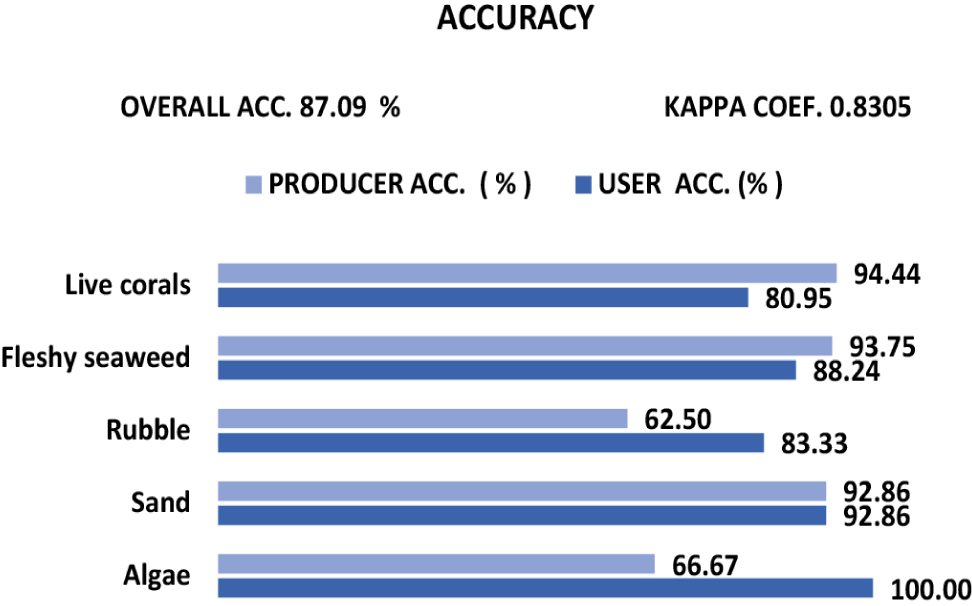
The accuracy calculation from the confusion matrix (Fig. 9) shows an overall accuracy of 87.09% and a kappa coefficient of 0.83. Besides the overall accuracy, the confusion matrix calculation also includes two accuracy types: user accuracy, which indicates how often classified pixels are correct within their assigned class, and producer accuracy, which measures how well the classification aligns with the reference data (Congalton & Green, 2019). The user and producer accuracy values for benthic habitats vary except for sand. Producer accuracy is the highest for live coral (94.4%), followed by Seaweed (93.8%), Sand (92.9%), Algae (66.7%), and Rubble (62.5%). For user accuracy, Algae is the highest at 100%, followed by Sand (92.9%), Seaweed (88.2%), Rubble (83.3%), and Coral (81.0%). Based on the classification results, the overall accuracy of the coral reef habitat using 62 ground checkpoints was 87.1%. Thus, this study was reasonably accurate.
Table 7 presents the calculated areas of each benthic habitat at the study sites on the Kadatua, Liwutonkidi, and Siompu Islands based on the MLH classification of Landsat-8 OLI imagery, as illustrated in Fig. 8. From this table, coral is the most significant area, followed by sand, seaweed, rubble, and algae. In contrast, the island with the largest habitat is Kadatua, followed by Siompu, and the lowest is Liwutonkidi. The area of Kadatua Island is much smaller, only 37.9 km2, than that of Siompu Island, 112.8 km2 (the Central Statistic Agency of South Buton Regency, 2024), while the coral cover of Kadatua, 173.2 ha, not that much different from Siompu around 186.2 ha. However, the rubble on Siompu Island (104.1 ha) is almost twice as high as that on Kadatua Island (56,7 ha). According to Haruddin et al. (2011), this high coverage of rubble on Siompu Island, particularly in BTNS-17 is directly proportional to the reports that many fishermen still catch the fish using explosives and potassium cyanide.
Table 8 presents the data collected from the fieldwork based on underwater photo transects of benthic live forms. The Hard coral (HC), which is composed of Acropora (AC) and non-Acropora (NAC), is considered quite reasonable based on the criteria of Giyanto et al. (2017) in Table 1 at the study sites of BTNC-D, BTNC-C, and BTNC-13 on Siompu, Liwutonkidi, and Kadatua Islands that have a percentage of HC > 35%, but on the other study sites like BTN-17 and BTNC-14 were classified as moderate, ranging between 19 and 35%. The combination of FS and dead coral with algae in all study sites is actually in moderate condition, but since the criteria of Table 2 are classified only into two classes of high and low, thus all moderate classes are classified as High.
The third criterion for the CHI is the density of coral reef biomass (kg/ha), as shown in Table 1. Thus, Table 9 lists the coral fish in all study sites. The coral reef fish consisted of two groups, the carnivorous and the herbivorous. The fish belongs to carnivorous include the families of Seranidae (Groupers), Lutjanidae (Snappers), Lethrinidae (Emperors or Scavengers), and Haemulidae (Grunts). Meanwhile, the herbivores are the families of Acanthuridae (Surgeonfishes, Tangs, and Unicornfishes), Scaridae (Parrot fish), and Siganidae (Rabbitfish). The total fish biomass density at the sampling locations from highest to lowest in order is BTNC-13 (895.2 kg/ha), BTNC-D (722.8 kg/ha), BTNC-C (446.9 kg/ha), BTNC-17 (391.7 kg/Ha) and the lowest BTNC-14 (329.3 kg/Ha). Based on the criteria of the CHI in Table 1, all the study sites fall outside the category of coral with high or medium health index because the RFB at all study sites was much lower than 940 kg/ha, so it is classified as low. The low RFB in all study sites was due to the lousy exploitation of reef fish by unfriendly fishing methods, mainly explosives and poison (Potassium cyanide; Haruddin et al. 2011).
Table 10 summarizes the calculation of the CHI based on the benthic live forms data collected during the underwater photos transect (Fig. 3 and Table 8) and RFB of the carnivorous and herbivorous (Fig. 4 and Table 9). According to the criteria of the CHI (Table 2), the CHI in the study sites ranges from value Index of 5 on the BTNC-17 (northern Siompu Island) and BTNC-14 (southern Kadatua Island) to Index value 6 on BTNC-D (southern of Siompu Island), BTNC-C (Liwutonkidi), and BTNC-13 (northern of Kadatua Island). The result of this analysis is mapped in Fig. 10. These CHI values of 5 were categorized as a little bit higher than poor, while 6 were classified as medium level, indicating that the coral reef was recovering. Hence, better management is needed to achieve better health conditions.
Discussions
This study discusses the mapping of coral reef habitats in Kadatua, Liwutonkidi, and Siompu Islands using Landsat-8 OLI satellite imagery data and further applies it to develop a CHI assessment. The standard procedures for satellite image processing are applied, such as corrections for atmospheric, sun glint, and water column influences. Habitat classification by applying the conventional method was then done using MLH (Fig. 1). The classification map consists of 5 classes, Algae, Coral, Seaweeds, Sand, and Rubbles, with the area for each class can be calculated (Table 7 and Fig 8) and the accuracy of the classification map is also determined (Fig. 9).
Regarding map accuracy, the accuracy value will be higher if the agreement between the classification results and field observations is higher (Hossain et al., 2020). Therefore, selecting an inappropriate ROI on each class representative can reduce the producer accuracy value, which indicates that all habitats generated from the image can be mapped well. Also, the user accuracy values show that the results of field observation of habitat classes can be used correctly in the mapping process (Hafizt et al., 2017).
In this study, the results of the simple classification of the coral reef habitat using Landsat-8 OLI image showed an overall accuracy of 87.2% within 62 ground truth points used, while based on the confusion matrix, the overall accuracy is 87.1%. The lowest accuracy is the producer accuracy of 62.5% for Rubble. Meanwhile, the lowest user accuracy of 81.0% is for corals and the kappa coefficient of 0.83. Based on the rules contained in Indonesian National Standard (SNI) of 7716:2011 (LIPI, 2014), the acceptable accuracy value for shallow seabed habitat mapping is ≥ 60%. According to Mumby et al. (1998), a 65-70% accuracy for mapping aquatic habitats using satellite sensing can be reasonably good. Furthermore, a 60-80% accuracy can be used to recommend natural resource monitoring inventory activities (Green et al., 2000). Therefore, in this study, the results of this classification for coral reef mapping were accurate enough and able to be used for various management purposes.
Regarding the condition of coral reef, such as percent of LCC based on the field observation using LIT method indicated that out of the five observation sites, four of them (BTNC-D/Kadatua Island, BTNC-C/ Liwutonkidi Island, BTNC-13 and -14/Siompu Island) were in moderate condition (LCC in the rages of 25–49.9%), except BTNC-17/Kadatua Island was in poor/bad condition (LCC < 25%). However, if the detailed analysis, such as Coral Mortality Index (CMI = % dead coral / % [Dead+Live corals]) and Coral Bio-Erosion Index (CBI = % HC / [HC + soft coral + Sponge + algae + other]) were computed using data in Table 8, with the criteria of both CMI and CBI of 0 –< 0.25 is quantified as 4; 0.24–0.50 as 3; 0.50–0.75 as 2; and > 0.72 as 1, then the sum of both criteria, resulting the ecological status of Very poor coral condition if the value: 0–2, Poor: 3–4, Good: 5–6 and Excellent: 7–8 (English et al., 1999; Zamani & Januar, 2020). Based on the above criteria and the computation, all the study sites are in the ranges of value 3 (BTNC-D, -C, and -14) and value 4 (BTNC-17 and -13). This fact revealed that the coral conditions in all observation sites are poor, which explains the tendency of HCs to shift into non-coral builder organisms, such as soft coral, sponges, algae, and others (Zamani & Januar, 2020). These poor coral conditions are strongly related to lousy fishing practices used by the fishermen, especially in BTNC-17 (Haruddin et al. 2011). Analysis of the CHI in Table 10 also showed that sites of BTNC-17 have the lowest CHI values of 5, followed by BTNC-14 of 5. These two sites also have the lowest RFB of < 400 kg/ha compared to the other observation sites.
Coral reefs are home to the world’s resources, and millions of people depend on coral for their livelihoods. However, local stressors and climate change have forced coral reefs to live under pressure (Souter et al., 2021). This study shows that the local stressors that most cause coral reef damage are destructive fishing practices, such as the use of explosives, cyanide, and environmentally unfriendly fishing gear that destroy coral reef structures and reduce biodiversity; in addition, the practice of taking coral for construction materials, decoration purposes, and the aquarium trade, weakening the ecosystem (Haruddin, 2011; Fig. 11). Furthermore, global stressors to coral reefs are caused by coral bleaching. Although there are no specific reports of coral bleaching events on the islands of Kadatua, Liwutonkidi, and Siompu, in general, coral bleaching has been observed in areas around those islands, such as the Wakatobi Islands, especially during El Niño events, which increases sea surface temperatures (SST) in 2010 and 2016 (Wouthuyzen et al. 2018). So, the coral bleaching events on the Kadatua, Liwutonkidi, and Siompu Islands, which are part of an ecosystem close to and similar to the Wakatobi Islands, are likely to cause coral bleaching.
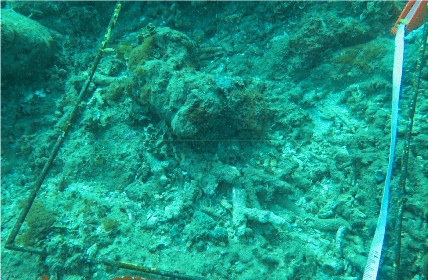
The explosives utilized to exploit coral reef fish can cause coral reef degradation characterized by low percentages of LCC, high dominance of rubble and algae, or even mass coral death (Fig. 11). Benthic algae will quickly colonize the dead coral reefs (Liao et al., 2021). This can be seen from the results of underwater photo transects in the benthic life form data of Table 8, where the combined components of rubble and dead coral covered with algae in almost all study locations are high, ranging from 50–60%. Still, at the study site in BTNC-17 (Siompu Island), it is the highest at 66.3%, as well as the cover of live coral reefs, is classified as poor (LCC is <25%). However, the other four locations are in moderate condition (25–50%).
Coral reef quality degradation is a painful truth, considering that the growth of coral is relatively slow (Fong & Todd, 2021; Morais et al., 2020), especially the Porites heronensis during the winter months (0.48 ± 0.04 mm per month) and Pocillopora damicornis during the summer months (1.18 ± 0.08 mm per month; Anderson et al., 2015). Corals that experience a decline in quality of life tend not to be able to provide ecosystem goods and services as they should. This study found that dynamite fishing to get fish is much more detrimental to coral reefs because reefs are home to resources that are needed by all living creatures. Damaged coral ecosystems are linear with low fish production, such as the condition in Fig. 11, which does not show any fish, even one. The high intensity of coral reef degradation in the long term will eliminate biodiversity, reduce fish catches, and ultimately place coastal welfare in an irreparable position, particularly for communities that depend on coral reef ecosystem services and marine resources (Benkwitt et al., 2020).
Reef fish coexist with coral reefs. Thus, the diversity and biomass of fish in coral reef ecosystems directly reflects the health of coral reefs. In this study, the biomass density of reef fish that consisted of 2 groups, the carnivorous (4 Families) and the Herbivorous (3 Families) (Table 9), was used to assess the coral reef’s health by applying the criteria of fish biomass density of > 1,940 kg/ha as the healthy coral reef environment, otherwise, < 940 as a poor condition, while in between those values as a medium condition (Table 1; Giyanto et al., 2017). The entire reef fish in all study sites was below the criteria (Table 9), which means that judging by coral reef fish abundance only, all coral reef environments in the study sites were in poor condition. Thus, the low coral fish below the criteria for healthy coral reefs due to dynamite and poison fishing that cause damage to benthic habitat and exacerbated by overfishing reveals facts that the coral conditions at the study sites are low health condition (Carvalho et al., 2021), such as at the BTNC-17 (Siompu Island) to moderate conditions for other study sites.
Table 11 lists the criteria for determining the health of coral reefs in the Caribbean waters of the Mesoamerican region (Mexico, Belize, Honduras, and Guatemala) based on the biomass of herbivorous and carnivorous coral fish (see the criteria in the notes below Table 11) as a comparison to the criteria developed by Giyanto et al (2017). Unlike the criteria of Giyanto et al (2017), in this criteria, the herbivorous fish used are limited to the surgeonfish group (family Acanturidae, especially from the species Acanthhurus spp and zebrasoma spp) and the parrotfish group (Family Scaridae, such as Cetoscarus spp; Chlorurus spp; Hipposcarus spp; Scarus Spp.). These Herbivorous fish are essential grazers in controlling the macroalgae that could overgrow the reef. Meanwhile, the carnivorous fish group is limited to fish from the family Serranidae (groupers) and Lutjanidae (Snapper). According to Table 11, the condition of coral reef fish from the Herbivore group is classified as high for BTNC-D and -13 and poor for BTNC-17, -C, and -14, while the Carnivore group is grouped as very high for BTNC-D, and -13, Poor for BTNC-17, and critical for BTNC-C and -14. Thus, the result of CHI determination based on Mesoamerican criteria, in general, is almost the same as Giyanto’s et al (2017) criteria for BTNC-17, -C, and -14 but the criteria for the Mesoamerican region seem more manageable to analyze, more detailed and reliable, and simpler than the criteria developed by Giyanto et al (2017), since it use only data of 2 groups of herbivore (Acanthuridae and Scaridae), and 2 groups carnivore fishes (Lutjanidae and Serranidae).
Herbivore fish (g/m2): Critical, <990; Poor, 990–< 1,860; Fair, 1,860–< 2,740; Good, 2,740–< 3,290; Very good, ≥ 3,290.
Carnivore fish (gram/m2): Critical, <390; Poor, 390–<800; Fair, 800–< 1,210; Good, 1,210–< 1,620; Very good, ≥ 1,620.
Data from McField et al., (2024)
In this study, it was seen that CHI was highly correlated with reef fish abundance. For example, although the CHI level in BTNC-D, -C, and -13 was 6, while BTNC-17 and BTNC-14 were 5, all study sites had a low fish abundance of < 970 kg/ha (Table 9) based on the criteria of Giyanto et al. (2017; Table 10). These results of CHI computation would be different if the fish abundance criteria from McField et al. (2024), were used (Table 11), which showed that BTNC-D and -13 had fish abundance classified as “Good for the Herbivorous fish group” and “Very good for the Carnivorous fish group”, while the abundance of coral fish in BTNC-17, -C and -14 were classified as “poor” and Critical” (Table 11). So, suppose the data in Tables 8 and 9 are reanalyzed using the criteria of McField et al. (2024); then, the analysis results reveal a more apparent difference in CHI of the two study sites (BTNC-D and -13), which have coral fish abundance in the categories “very good” and “good”, where the CHI in both locations is also classified as “very good” (Table 12). In contrast, the remaining 3 study sites (BTNC-17, -C and -14) with coral fish abundance in the categories “poor and Critical” have CHI values classified as “fair/moderate (Table 12).
From the results of this analysis, it can be considered that the McField et al. (2024) criteria, such as in Table 12, are more reliable to be applied in determining the CHI in each study site and supporting the explanation of reef fish abundance than the Giyanto et al. (2017) criteria in Table 2, which classifies CHI with a wide range level from 10 to 1. Level 10 is the healthiest coral reef, with a high percentage of LCC and coral resilience, thus supporting abundant reef fish. Conversely, CHI level 1 is a coral reef with the lowest LCC and resilience, making it difficult for corals to grow and develop, resulting in a low abundance of economically valuable reef fish. Furthermore, there is no specific information about CHI for levels outside of the ranges from 10 to 1, for example, levels 9 to 2. So, it isn’t easy to get detailed information on the status of the CHI.
The quantity and quality of LCC illustrate the level of resilience and affect how the benthic components survive. Corals with high levels of resilience have good adaptability when faced with disturbances and pressures. From Table 10, it can be seen that the coral resilience in the study sites is high, as indicated by the low fleshy algae cover (– 0%). However, the coral RFB based on Giyanto’s et al (2017) criteria was low, while LCC varies from poor conditions, such as in BTNC-17, to moderate in other locations. The results of this study produce relatively a low CHI of 5 (BTNC-17 and -14), but a slightly high of 6 (BTNC-D, -C and -13, Table 13). Table 13 also shows that the CHI in this study was lower compared to the CHI of 2016 as in BTNC-14 from a level of 6 to 5. However, there were also increases, such as BTNC-D from a level index of 5 to 6, while the remaining BTNC-C and -13 had the same level of 6 both in 2016 and 2021 including BTNC-17 that surprisingly remain the same as in 2016. Therefore, the CHI on the study sites, in general, tends to decrease, but some exceptions show also improvement, such as in BTNC-D or remain the same as 2016. Despite high coral resilience indicated by low fleshy algae presence (resilience potency), the overall CHI remains impacted by low coral RFB and variable of coral cover conditions.
Data from Giyanto et al. (2017).
To address this decline, particularly for the study sites, several efforts can be made as follows: (1) To control lousy fishing practices and overfishing in these study sites by implementing and enforcing sustainable fishing to maintain the balance of marine life; (2) To reduce marine pollution by limiting the discharge of pollutants, including sewage, agricultural runoff, and sedimentation into the ocean. (3) To allow coral reefs to recover and thrive without human interference, e.q. by establishing marine protected areas (MPA) or No-Take Zone areas; (4). To Engage in coral restoration projects, such as coral gardening and transplantation, to help damaged reefs recover; (5). To educate and involve the local communities in conservation efforts to ensure long-term sustainability and protection of coral reefs. These efforts can help improve the CHI and ensure the long-term health and resilience of coral reef ecosystems.
Special efforts must be emphasized to rehabilitate the coral reef degradation, especially in the three sites, the BTNC-17, -14, and -C, followed with the kind effort from the above recommendation of points 1, 2, and 5, but firstly by starting the establishment of the No-take zone or MPA (point 3) and conducting coral transplantation (point 4). The No-take zone/MPA established by the local community has proven effective in recovering both the reef condition and reef fish population in the 20 sites of the small Islands of the Biak-Numfor and Supiori Districts in the Gulf of Cendrawasih, Papua in 2009–2014. The abundance of reef fish inside the No-take zone was 3–4, 3–5, and 2–3 times higher than the outside for the target/commercial fishes: the fish being the catch target by fishers, indicator fish, the butterfly fish of the family Chaetodontidae, which can indicate the health of the coral reefs; and major fish group, the relatively small size fish that are mostly grouped as ornamental/aquarium fishes, respectively (Wouthuyzen et al. 2016). The two study sites that show good/excellent CHI, like BTNC-D and -13 (Table 12), are also better if the No-take zone is established there. It is hoped that the reef fish from the No-take zones can spill over to the surrounding sites or outside the established no-take zone.
Conclusions
This study assesses the CHI using Landsat-8 OLI remote sensing and in-field LIT surveys. The Landsat-8 data effectively mapped benthic habitats, including coral, macroalgae, sand, and rubble, with – 81% overall accuracy. The LIT surveys provided data on LCC, fleshy macroalgae as a resilience indicator, and reef fish abundance (using UVC, Fig. 4), which were used to determine the CHI.
Based on the Giyanto et al. (2017) criteria, CHI was categorized into two levels: level 5 (BTNC-14 and -17) and level 6 (BTNC-13, -C, and -D). A comparison between 2016 and 2021 revealed a decline in CHI for BTNC-14 (level 6 to 5) and an improvement for BTNC-D (level 5 to 6), while other sites remained at level 6. However, distinguishing whether levels 5 and 6 indicate good or poor conditions remains challenging. Reef fish abundance was low (<970 kg/ha) across all sites, with BTNC-14, -D, and -C having the lowest values (<500 kg/ha), which is related to destructive fishing practices.
CHI was also compared using McField et al. (2024) criteria applied for annually monitoring the coral reefs in Mesoamerican (Mexico, Belize, Guatemala, and Honduras) countries from 2006 to 2023. This method classified BTNC-13 and -D as “very good/excellent” and BTNC-C, -17, and -14 as “fair.” McField’s criteria provide a more precise, reliable framework that is simpler for assessing CHI and explaining reef fish abundance, making them a viable alternative for monitoring Indonesia’s coral reef ecosystems.
Based on these findings, several key recommendations are issued: (1) Establish a MPA by designating a small no-take zone of about 1 to 10 ha at each study site to protect the coral reefs, and allow the fish population to recover, and enhance fish spillover into surrounding areas (this approach has proven successful in Biak Island, Papua; Wouthuyzen et al. 2016). (2). Implement coral transplantation/coral gardening, particularly in sites with poor or fair CHI levels, such as BTNC-14, -17, and -C. (3). Regulate fishing practices by enforcing sustainable fishing regulations to curb overfishing and destructive methods like blast and cyanide fishing, and ensure marine life balance. (4). Reduce marine pollution by minimizing the discharge of pollutants, including sewage, agricultural runoff, and sedimentation, to improve water quality and support reef resilience. (5). Enhance community involvement and monitoring by conducting long-term research and involving local communities in conservation initiatives to promote awareness and sustainable reef management.
Those recommendations provide a roadmap for improving reef health and ensuring the long-term sustainability of coral ecosystems in the Kadatua, Liwutonkidi, and Siompu Islands. Therefore, this study’s findings can serve as a benchmark for monitoring future changes in the coral reef environment.