Length-weight relationship and condition factors of native freshwater fishes in the Hajar Mountain, Oman

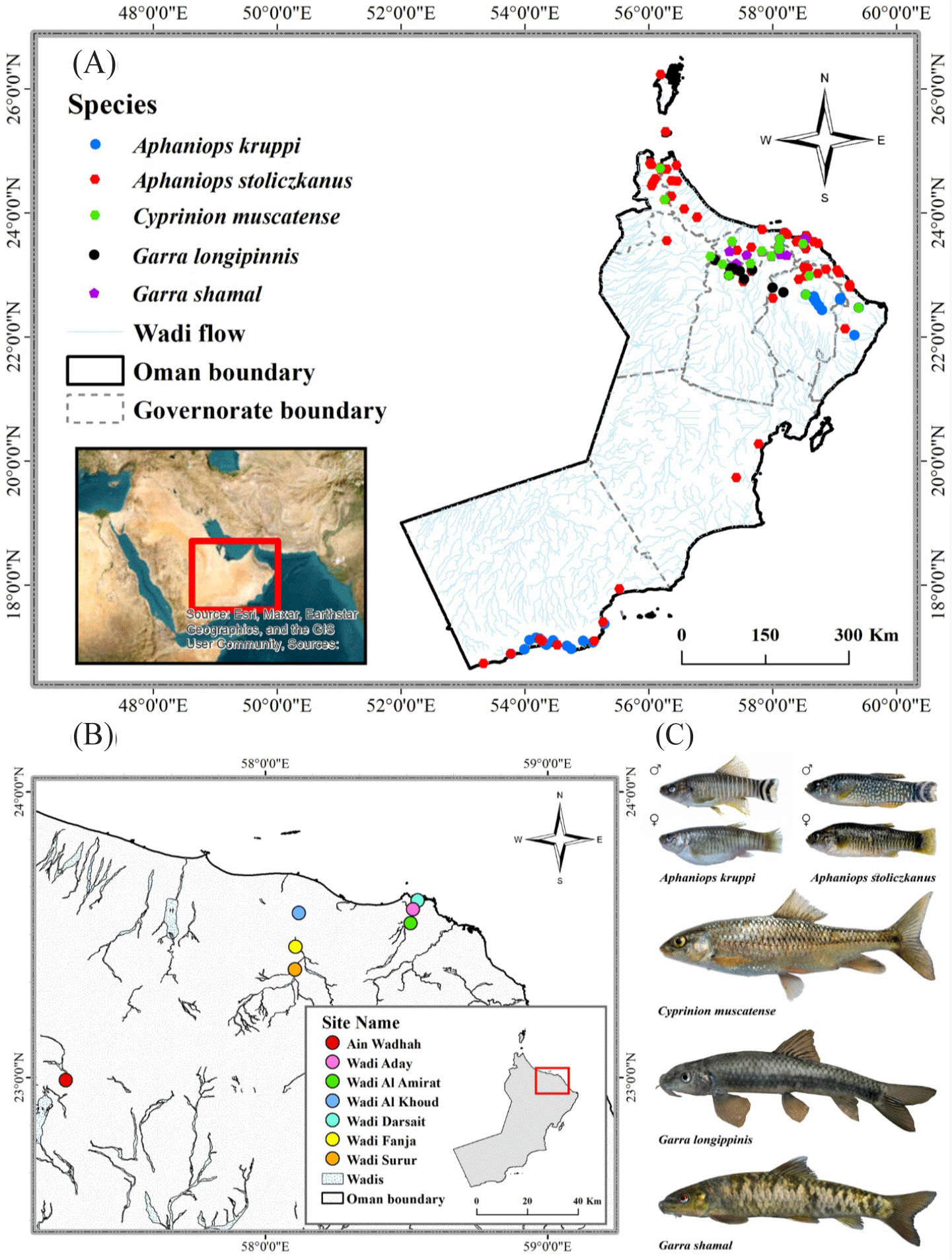
Oman is located in the south-eastern part of the Arabian Peninsula (Fig. 1). Omani climates are characterized by arid interiors dominated by the Rub al Khali desert, as well as semi-arid regions along with parts of the Omani coasts near the Hajar Mountains (Beshkani et al., 2017). The Hajar Mountains are distinguished by a diverse geological composition. Despite the aridity of the region, the Hajar Mountains present a climatically unusual setting in comparison to the neighboring areas. The elevated peaks, profound canyons, and distinctive topography of the Hajar Mountains generate a range of ecological habitats, rendering the area an optimal site for the existence of endemic flora and fauna species (Carranza et al., 2021). The Oman Mountains, specifically the Hajar Mountain range, are recognized as a freshwater ecoregion (ID 443) by the World Wildlife Fund for Nature (WWF) (Abell et al., 2008). There are several wadis (spring-fed watercourses) in the Hajar mountain range proving natural habitat for fish, despite the limited precipitation in the area (Burt, 2003). This study was carried out in seven wadis, a bed or valley of water stream, located in the Hajar Mountain range in northeastern Oman. All of these sites originate from the Hajar Mountain ecoregion with permanent streams throughout the year. Additionally, all sites are accessible with presence of native freshwater fishes. Fish were collected in March 2023 (spring) for the study from the following sites: Ain Wadhah (AW; 22°59’N, 57°17’E), Wadi Aday (WA; 23°35’N, 58°31’E), Wadi Al Amirat (WAA; 23°32’N, 58°30’E), Wadi Al Khoud (WAK; 23°34’N, 58° 07’E), Wadi Darsait (WD; 23°37’N, 58°32’E), Wadi Fanja (WF; 23°27’N, 58° 06’E), and Wadi Surur (WS; 23°22’N, 58° 06’E) (Fig. 1).

Fig. 1. Distribution and diversity of freshwater fishes in Oman. (a) Geographic occurrence of five species across the Oman’s wadi network; (b) sampling locations across seven wadis in Hajar Mountains, Oman; and (c) morphological characteristics of studied species.

Download Original Figure

The study covered multiple species, each found in different water bodies across the Hajar mountain region. The method employed for capturing fish samples involved the utilization of foldable shrimp and crab fishing traps (with a mesh size of 3 × 3 mm, comprising 4 nets left in the watercourse for a standardized duration of 5 h; Supplementary Fig. S1 and S2) (Al Jufaili et al., 2021; Bidaye et al., 2023; Güçlü et al., 2021, 2024; Masoumi et al., 2023). The sampling equipment chosen is effective in a location where fish could enter traps but not exit. The fish species identified within the sampling sites included 3 endemic fish species Aphaniops kruppi (Freyhof et al., 2017), Garra longipinnis (Banister & Clarke, 1977), and Garra shamal (Kirchner et al., 2020). Moreover, 2 native fish species C. muscatense (Boulenger, 1888), and Aphaniops stoliczkanus (Day, 1872) (Esmaeili et al., 2022; Freyhof et al., 2021) were also identified in the sampling sites (Fig. 1). The collected specimens were preserved in a 70% alcohol solution. A digital caliper (INSIZE Caliper 300 MM, INSIZE, Suzhou, China) with an accuracy of 0.01 mm was used to measure the total length (TL) (Güçlü et al., 2024; Masoumi et al., 2023) from the front of the snout to the upper lobe of the caudal fin (Carlander & Smith Jr, 1945). The specimens were subjected to a weighing procedure with a precision of 0.01 g (total weight, TW) using a digital electronic balance (Precisa PB 320M Analytical Laboratory Balance, Precisa, Dietikon, Switzerland).

The relationship parameters between the length and weight were estimated by using the power function formula: W = aL^b, where W is the total weight, L is the length, a is the intercept, and b is the slope of the log-transformed data (Froese, 2006; Güçlü et al., 2024). The strength of the relationship between the length and weight variables was quantified using the coefficient of determination, R². Moreover, the 95% confidence intervals of a and b were estimated (Morey et al., 2003). Before conducting the regression analysis, log-log plots of length and weight values were used to visually identify outliers (Al Jufaili et al., 2021; Froese, 2006). The statistical significance of the length-weight relationships for the fish species was evaluated using analysis of variance (ANOVA). To determine whether the b-value (slope) significantly deviates from the expected cube value of 3, Bailey’s t-test formula (t = [b – 3] / S_b) was used, where b is the slope (b-value) obtained from the linear regression and Sb is the standard error of the slope (p = 0.05; Morey et al., 2003). The exponent b indicates growth patterns: b ≈ 3 for isometric growth, b > 3 for positive allometric growth, and b < 3 for negative allometric growth (Morey et al., 2003). Isometric growth is when weight increases directly with length. Values of b greater than 3 indicate disproportionately heavier bodies (relative to length) and values less than 3 indicate slimmer bodies (Tesch, 1978).

Fulton et al. (1911), Tesch (1978), and Le Cren (1951) equations were used to estimate Fulton’s condition factor Kc = 100 × W/L³, allometric condition factor Ka = 100 × W/L^b, and relative condition factor Kn = W/aL^b, respectively. In the equations, a is the intercept, b is the regression coefficient, L is the total length, and W is the total weight. A Kc evaluates the general health, growth, and reproduction of a fish (Froese, 2006; Jisr et al., 2018). Ka determines if a fish’s growth is isometric or allometric (Froese, 2006). Le Cren (1951) introduced the Kn as a way to compare a fish’s observed weight with its expected weight based on the length-weight relationship. A value of 1 for Kn indicates average condition. For statistical analysis and graph plotting, Microsoft Excel and Origin Pro OriginLab were used.

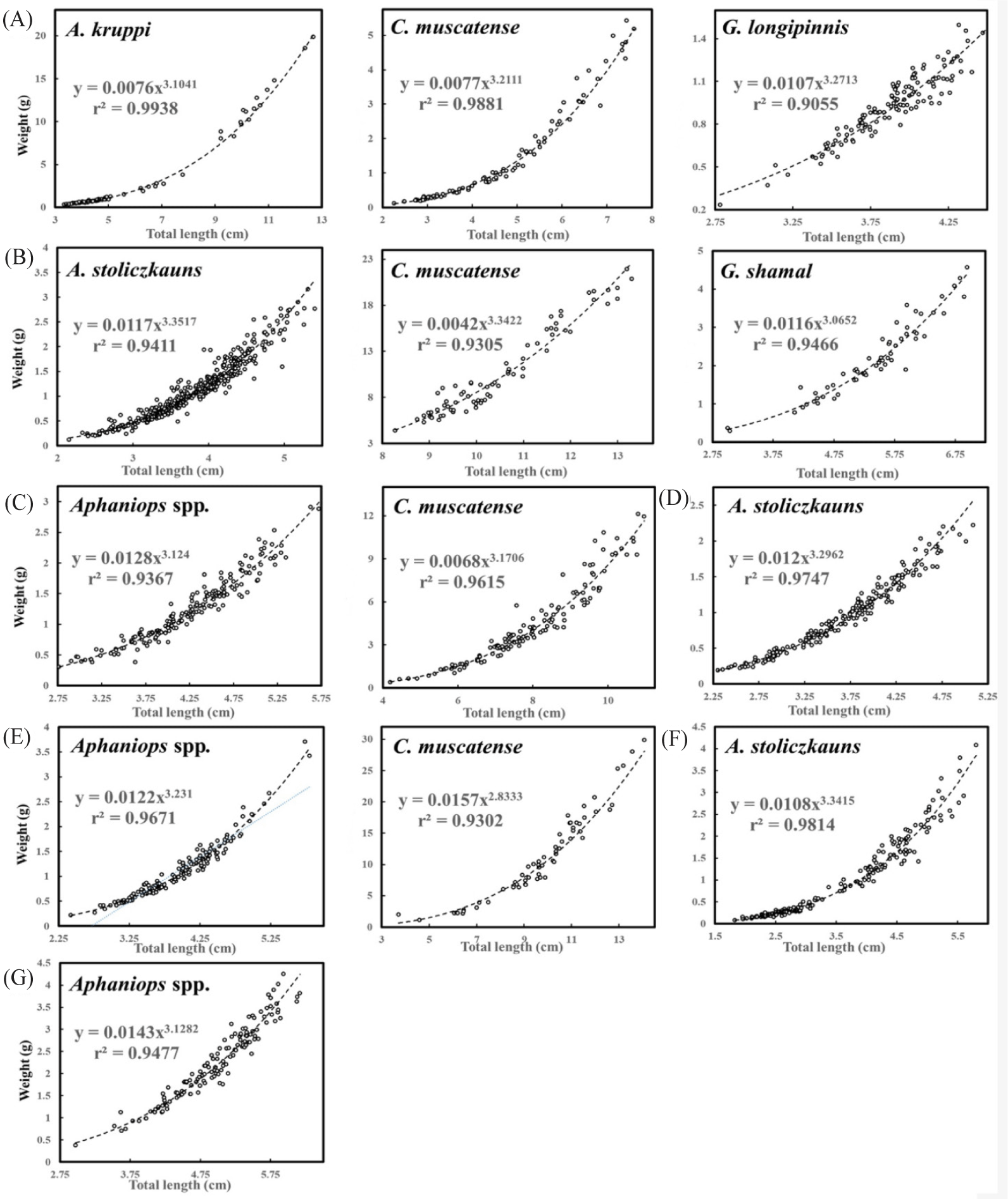
Sample sizes varied across species and locations, ranging from 59 to 402 individual fish, indicating a reasonably robust dataset for analysis (R² ≥ 0.906; Table 1 and Fig. 2). The LWR parameters, represented by coefficients a and b and their 95% confidence interval (CI), the coefficient of determination (R²), and the growth type were calculated for each species and location (Table 1). Significant LWRs were observed across all species (p < 0.001). The range of values for b extended from 2.833 to 3.357, falling within the anticipated range of 2.5 to 3.5 (Froese, 2006). Freshwater fish species in (Fig. 2) show a positive length-weight correlation with varying strength indicated by different R² values (Froese, 2006). The above values are centered on the collective genders of the studied fish species.

Fig. 2. Length-weight relationships of five freshwater fish species (combined sex) collected from different wadis in the Hajar Mountain, Oman. (A) Ain Wadhah (AW); (B) Wadi Al Amirat (WAA); (C) Wadi Al Khoud (WAK); (D) Wadi Aday (WA); (E) Wadi Surur (WS); (F) Wadi Darsait (WD); (G) Wadi Fanja (WF).

Download Original Figure

These parameters provide insights into the relationship between the length and weight of the fish. Higher R² values suggest a better fit of the model to the data (Jisr et al., 2018). Bailey’s t-test illustrated that b-values significantly deviated from 3, except for C. muscatense located in WS, potentially due to constraints in sample size, ontogenetic changes (Froese, 2006), reproductive status (Cone, 1989), environmental conditions, genetic factors, and sampling bias (Froese, 2006; Ragheb, 2023). Variability within species persists across different locations (Famoofo & Abdul, 2020). Regression equations by Ricker (1973) predict weight from length for each species, crucial for growth patterns, biomass estimation, and population dynamics in the Hajar Mountain region (Hilborn & Walters, 2013). These relationships reflect diverse environmental impacts on fish growth in sampled wadis (Beverton & Holt, 2012).

The b-value of the LWR among various fish species in the Hajar Mountain region of Oman in TL, as documented in (Table 1) displays notable variations compared to the findings presented by Al Jufaili (2021). Within the species A. stoliczkanus, the b-values listed in the table span from 3.104 to 3.352 for males and 3.282 to 3.419 for females at different locations, diverging from the values of 2.882 for males and 4.150 for females as outlined by Al Jufaili (2021). Similarly, for A. kruppi, the table illustrates b-values ranging from 3.790 for males and 3.177 for females, contrasting with the values of 2.811 for males and 2.985 for females reported by Al Jufaili (2021). Furthermore, the table indicates a b-value of 3.211 for G. longipinnis, which closely aligns with the value of 3.104 documented by Al Jufaili (2021). Conversely, the b-values for C. muscatense vary from 3.104 to 3.342 in the table, deviating from the value of 2.974 presented by Al Jufaili (2021).

The study tested the hypothesis that a b-value of 3 represents isometric growth (I), with length and weight increasing proportionally. When b is above 3, it indicates positive allometry (+), showing weight increases faster than length. Contrariwise, if b is below 3, it suggests negative allometry (–), where weight increases slower than length. The analysis of the differences in LWRs among species revealed the following outcomes: A. kruppi at AW, G. longipinnis at AW, and A. stoliczkanus at WA, WAA, and WD exhibited positive allometric growth (b > 3), suggesting that these species tend to become relatively heavier as they increase in length. This phenomenon could be attributed to alterations in body shape, augmented reproductive organs, or the accumulation of energy reserves (Hossain & Sultana, 2014). Furthermore, G. shamal at WAA displayed isometric growth (b ≈ 3), indicating a proportional augmentation in both length and weight, which is a common characteristic in numerous fish species (Froese, 2006). The mix growth patterns of isometric and positive allometric growth in C. muscatense and Aphaniops spp. might be influenced by a variety of factors such as habitat, feeding behaviors, or reproductive strategies. Generally, the differences observed in LWRs among various fish species can be attributed to a multitude of factors, such as dissimilarities in research sites, environmental factors, food availability, disease, and competition (Al Jufaili et al., 2021; le Cren, 1951; Tesch, 1978). The complex interplay of these variables may lead to discrepancies in the determined LWRs. These findings illuminate the diverse growth patterns manifested by fish species within the Hajar Mountain region, emphasizing the significance of incorporating ecological components into the comprehension of their growth dynamics (Froese, 2006).

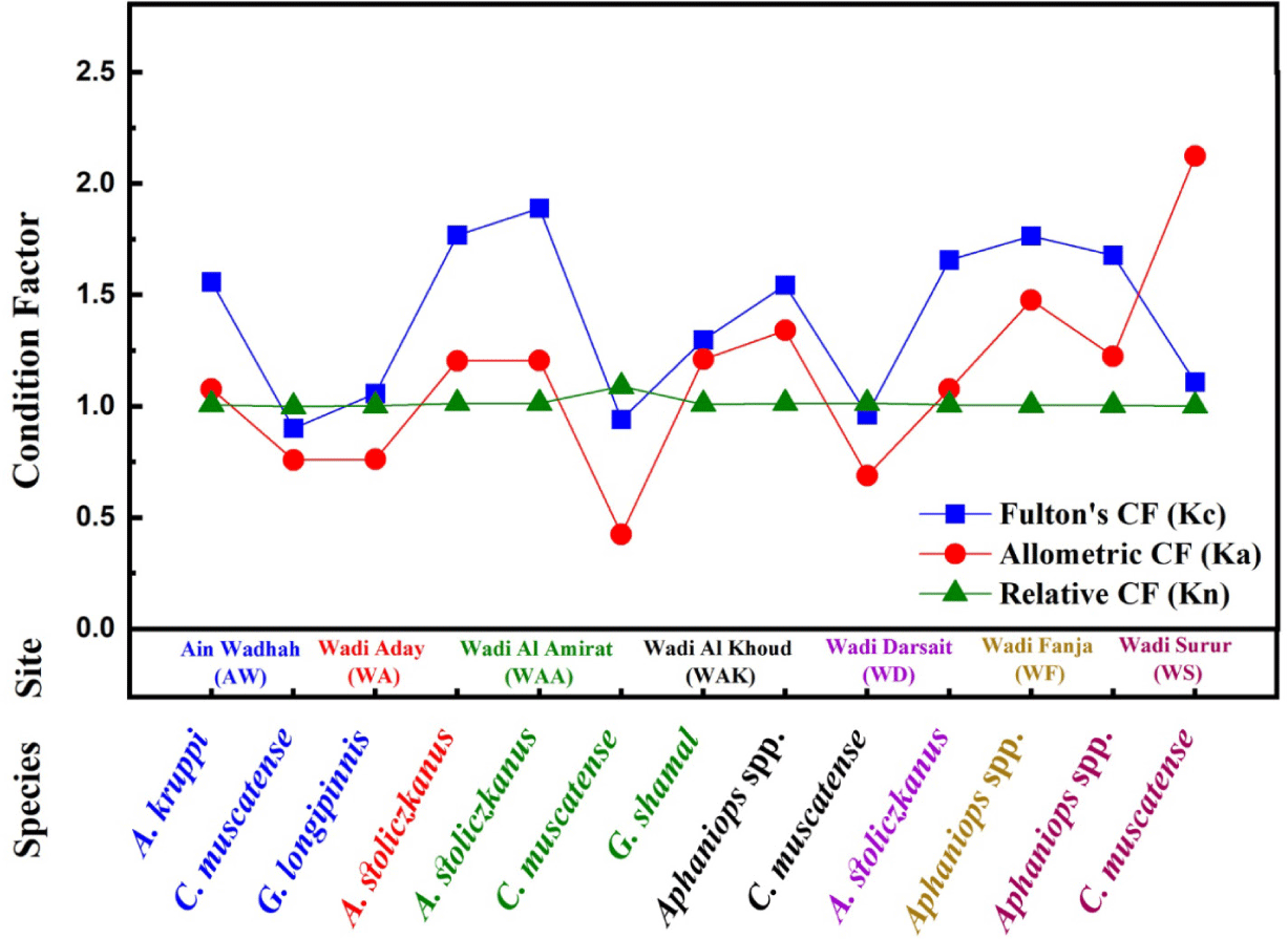
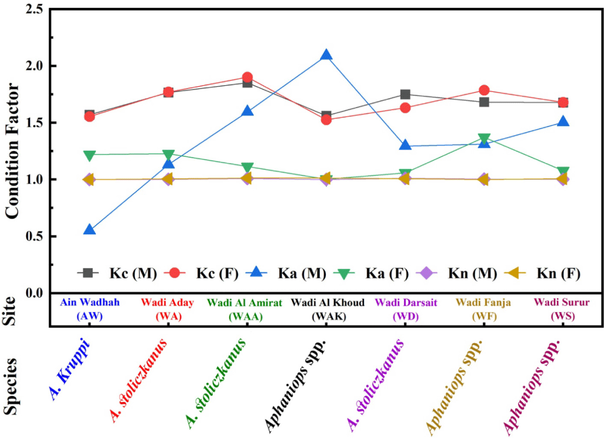
Table 2 presents Kc, Ka, and Kn for the fish species delineated in Table 1, this data illustrates the range and mean values of each factor across various species, sexes, and locations, thereby enabling comparative analyses. Figs. 3 and 4 graphically depicts the condition factors across different sites, sexes, and species, aiding in the detection of noteworthy findings.

Fig. 3. Comparison of condition factors across seven wadis in the Hajar Mountains, Oman. Kc, Ka, and Kn for five fish species (combined sex). Kc, Fulton’s condition factor; Ka, allometric condition factor; Kn, Relative condition factor; AW, Ain Wadhah; WA, Wadi Aday; WAA, Wadi Al Amirat; WAK, Wadi Al Khoud; WD, Wadi Darsait; WF, Wadi Fanja; WS, Wadi Surur.

Download Original Figure

Kc is used to assess fish species’ well-beingness, even with allometric growth and b ≠ 3 (Ragheb, 2023). The mean Kc values exhibit significant variations among the fish species, sites, and sexes, with a range from approximately 0.902 ± 0.085 to 1.889 ± 0.288. The most elevated Kc values across diverse fish species manifest in A. stoliczkanus at WAA (combined: 1.889 ± 0.288; females: 1.901 ± 0.299, males: 1.8513 ± 0.245), Aphaniops spp. at WF (combined: 1.766 ± 0.174; females: 1.786 ± 0.171, males: 1.682 ± 0.165), A. kruppi at AW (combined 1.559 ± 0.138; males: 1.570 ± 0.147, females: 1.554 ± 0.135), and G. shamal at WAA (1.299 ± 0.167). These values suggest these species are in superior physical condition, possibly due to factors like food availability, reproductive status, or environmental conditions. (Froese, 2006). Moreover, across various locations, A. stoliczkanus generally showed higher average Kc values, suggesting better condition compared to other species. On the other hand, C. muscatense and G. longipinnis displayed lower Kc values compared to the other species. The average Kc values for C. muscatense were less than 1.0 at locations AW, WAA, and WAK: 0.902 ± 0.085, 0.941 ± 0.111, and 0.963 ± 0.141, respectively.

The Ka values indicate the growth pattern observed in the length-weight relationships. The highest mean Ka value, 2.124 ± 0.556, was recorded for C. muscatense at WS, as illustrated in Table 2 and Fig. 3. This particular outlier requires further investigation to determine its origin, whether from measurement errors or unique environmental conditions at that specific location. Nevertheless, this data implies a superior state of well-being for this species at the mentioned site, based on the allometric condition factor. Species displaying positive allometric growth, such as A. kruppi and A. stoliczkanus, exhibit higher Ka values, while C. muscatense presents lower Ka values. This species had the lowest mean Ka value, 0.425 ± 0.048 at WAA, indicating a relatively lower condition at this site. Aphaniops spp. generally displayed higher mean Ka values across sites, for example, 1.477 ± 0.144 at WF and 1.341 ± 0.153 at WAK, suggesting a better condition based on the allometric factor compared to other species.

Table 2 and Fig. 4 displayed a significant sexual differentiation in Aphaniops spp. at WAK (males: 2.090 ± 0.234, females: 1.003 ± 0.131), possibly due to sex-based differences in habitat use or sex-specific feeding strategies. Moreover, A. Kruppi presented inverted patterns (males: 0.550 ± 0.041, females: 1.220 ± 0.106), indicating that energy allocation strategies differ between species (Froese, 2006; Mainero et al., 2023). These variability in Ka values suggests differences in the length-weight relationships and growth strategies among the fish species, attributable to variations in environmental conditions like water quality, temperature, and flow regime (Froese, 2006). Furthermore, factors such as food availability, habitat complexity, and resource competition can impact the condition and growth patterns of fish (Mainero et al., 2023). Biological aspects including reproductive status, age distribution, and genetic diversity within populations could also contribute to the observed variations in Ka values (Cone, 1989).

Fig. 4. Comparison of condition factors across seven wadis in the Hajar Mountains, Oman. Kc, Ka, and Kn condition factors for M and F Aphaniops species. Kc, Fulton’s condition factor; Ka, allometric condition factor; Kn, relative condition factor; M, male; F, female; AW, Ain Wadhah; WA, Wadi Aday; WAA, Wadi Al Amirat; WAK, Wadi Al Khoud; WD, Wadi Darsait; WF, Wadi Fanja; WS, Wadi Surur.

Download Original Figure

Mean Relative Condition Factor values typically cluster around 1, which is common for healthy fish populations (Kim et al., 2023; Le Cren, 1951), showing remarkable consistency between genders for females and males. Certain species like C. muscatense at WAA with a mean Kn of 1.090 ± 0.123 show deviations with a slightly higher condition compared to the population average. Instead, the lowest mean Kn value of 0.999 ± 0.086 was observed for C. muscatense at AW, indicating a relatively lower condition compared to the overall population.

This variability in Kn, especially in C. muscatense, suggests potential differences in nutritional status or habitat conditions across study sites (Jisr et al., 2018; le Cren, 1951). Largely, most species at different sites showed mean Kn values close to 1, suggesting similar conditions to the overall population. Kc typically exhibits elevated values when compared to the Ka and Kn, suggesting a potential tendency to overestimate the condition of fish populations. According to Froese (2006), Fulton’s condition factor assumes isometric growth, where length and weight increase proportionally, a scenario often not reflected in reality. Consequently, Kc may overstate the condition, particularly for larger or older individuals characterized by slower weight gain relative to their length. Conversely, the allometric condition factor (Ka) and relative condition factor (Kn) consider the allometric growth pattern, where weight increases at a different rate than length, and assess the individual’s condition against a reference population, respectively. These indices are deemed more precise in evaluating the condition of fish populations. Furthermore, the decrease in condition factors at the beginning of spawning in freshwater fish in Oman may be due to high metabolic rates (Lizama & Ambrosio, 2002). Variations in condition factors of C. muscatense and G. longipinnis may align with this reasoning (Table 2 and Fig. 3). Spawning periods of freshwater fish in Oman lack thorough documentation. However, freshwater fish near Oman, like those in Iran, typically spawn during spring (Mostafavi et al., 2021). Thus, using all three condition factors together gives a comprehensive evaluation of fish health, growth patterns, and environmental influences. Interpretation of condition indices should also include factors like reproductive cycle, and feeding behavior.