A Bayesian state-space production model for Korean chub mackerel (Scomber japonicus) stock

Introduction

This study is the first attempt to apply a Bayesian state-space production (SSP) model to Korea chub mackerel (Scomber japonicus) population, which is a coastal-pelagic fish species distributed in a wide range of depths from the surface to continental slopes, down to around 300 m in warm and temperate waters (Castro Hernández & Ortega Santana, 2000). Given the data about annual yield from all fisheries, and annual catch-per-unit-effort (CPUE) collected from the large purse seine fishery, we chose a state-space surplus production model. Previous assessments for the population (e.g., Cho et al., 2009; Choi et al., 2004b; Choi et al., 2004a did not consider process errors in their analysis.

Surplus production models or biomass dynamics models have been studied because of their advantages over other assessment models. These advantages include simpler model structures and fewer model parameters to estimate (Carruthers et al., 2011; Chaloupka & Balazs, 2007; McAllister et al., 2001; Millar & Meyer, 2000b; Pedersen & Berg, 2017). Management reference points, such as the maximum sustainable yield (MSY) and the biomass that yields MSY are estimated (Prager, 1994; Punt, 2003). Despite these benefits, biomass dynamics models have been criticized for aggregating growth, recruitment, and natural mortality into a surplus production term, at the cost of biological realism (Millar & Meyer, 1999).

de Valpine (2012) proposed that a more realistic model provides a better estimation. Since a stock assessment model is a simplified version of a dynamic system, and fits fisheries data that are generally noisy, the variability should be considered for both the model and the data (Aeberhard et al., 2018). Adopting a state-space framework for production models can mitigate the simplicity of production models by incorporating process errors and observation errors. Process errors in a biomass dynamics model describe uncertainties of random effect parameters such as biomass, and observation errors account for the noise in the data. Despite the ability to account for these two sources of uncertainty, the inclusion of process errors requires the estimation of a number of free parameters, and high-dimensional integration. Over the past few decades, researchers have implemented state-space models under assumptions such as model linearity, which is ecologically unrealistic, within the frequentist statistical approaches. The development of statistical software such as ADMB-RE (Fournier et al., 2012; Skaug & Fournier, 2017) and TMB (Kristensen et al., 2016) has enabled the implementation of state-space models with Gaussian error structure using the Laplace approximation. Another advantage of ADMB-RE is that the program provides Markov Chain Monte Carlo (MCMC) sampling without any revision of the computer code. Because the numerical optimization of parameters could not be achieved without priors, we specified prior distributions to stabilize the numerical optimization.

Using the ADMB-RE software for implementing Bayesian SSP models, we estimated the annual biomass, intrinsic growth rate carrying capacity, and associated uncertainties. We further provided management reference points, including MSY, biomass that yields MSY (B_MSY), and harvest rate that corresponds to MSY (H_MSY). We also compared the performance of our model with those of others.

Methods

Data

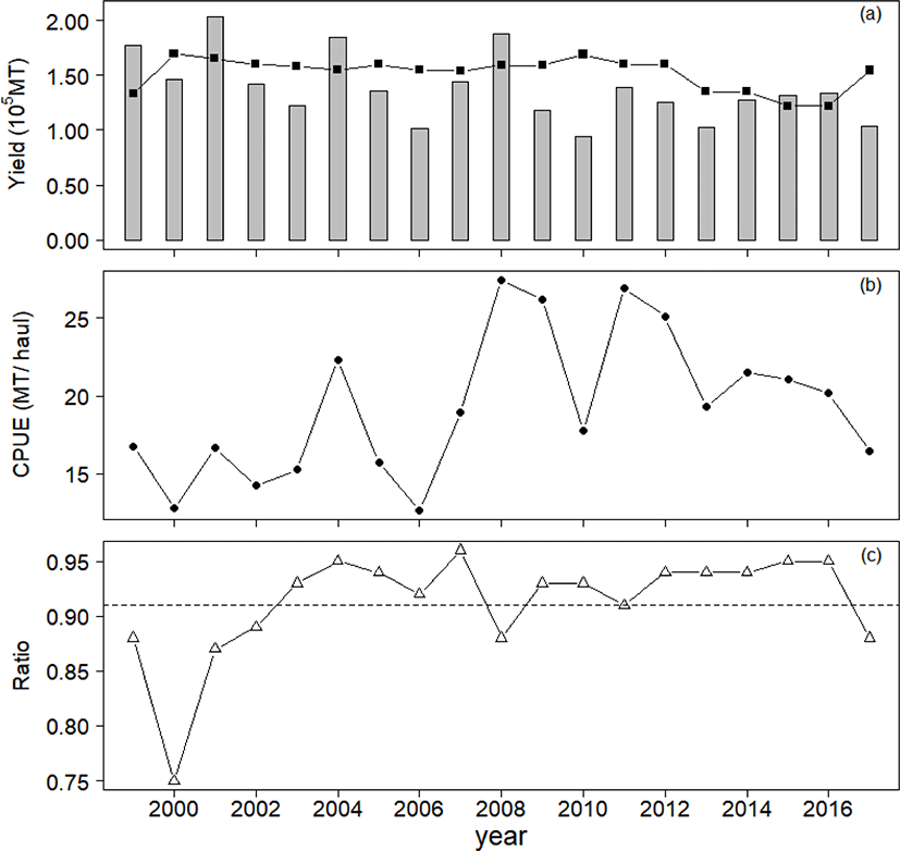
Two sets of historical data were used in this study: annual yield and catch-per-unit-effort (CPUE) for chub mackerel collected from Korean waters from 1999 to 2017 (Fig. 1). The Korean National Institute of Fisheries Science provided standardized CPUE with yield and effort data for 70% of the total large purse seine fisheries in Korea. We considered the chub mackerel CPUE (Fig. 1b) to be representative of all chub mackerel fisheries, as large purse seine fisheries accounted for more than 90% of the total on average (Fig. 1c).

Fig. 1. Historical data on Korean mackerel. Bars in panel (a) shows the yield of chub mackerel caught by the large purse seine fisheries, and line on squares indicates the total allowable catch. Panel (b) shows the annual CPUE collected from the large purse seine fisheries. Panel (c) shows the ratio of yield from the large purse seine fisheries to the total yield from all chub mackerel fisheries. In panel (c), the broken horizontal line indicates the mean ratio of yield from the large purse seine fisheries to total yield from 1999 to 2017. CPUE, catch-per-unit-effort.

Download Original Figure

Results

With the specified priors and data about yield and CPUE, we obtained posterior distributions for each parameter (r, k, q, ${\sigma }_p^2$, ${\sigma }_o^2$, P₁₉₉₉) using MCMC samples. We determined our MCMC samples built converged posterior distributions for each parameter (r, k, q, ${\sigma }_p^2$, ${\sigma }_o^2$, P₁₉₉₉), while accounting for the diagnostic results provided in Table 2. For each sample set of parameters, the dependence factor of the Raftery-Lewis statistics was around 1, the lag-1 correlation was around 0, the ratio between naïve and time series standard errors was around 1, and the posterior distribution was unimodal (Table 2 and Fig. 2).

Fig. 2. Prior probability distribution (dotted line) for parameters r, k, q, ${\sigma }_p^2$, ${\sigma }_o^2$, P₁₉₉₉, and posterior probability distribution (histogram) obtained from Markov Chain Monte Carlo sample sets. We specified log-normal priors for r and k and P₁₉₉₉, inverse gamma priors for ${\sigma }_p^2$ and ${\sigma }_o^2$, and uniform priors for log q. Units of k and q are metric tons (MT), and 1/haul, respectively.

Download Original Figure

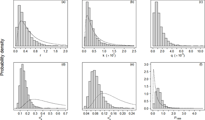
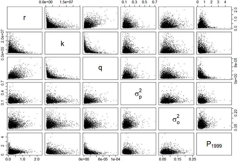
The estimates (posterior modes) of intrinsic growth rate r, carrying capacity k, and catchability q were 0.16, 1,832,623 metric tons (MT), and 5.49 × 10⁻⁵ haul⁻¹, respectively. The CV of the process error was nine times larger than that of the observation error, calculated as 84% and 9%, respectively. Based on the estimates of r and k, the calculated management reference points MSY, B_MSY, and H_MSY were 152,677 MT, 910,866 MT, and 0.08, respectively. Table 3 lists the 95% credible intervals for each parameter. Based on the scatter plots of joint posterior samples for both parameters, r and q exhibited negative relationships with k (Fig. 3). The former relationship can arise when the stock is large with low productivity, or small with high productivity (Millar & Meyer, 2000b; Walters & Martell, 2004). Millar & Meyer (2000b) also mentioned that the carrying capacity k in equation (2) scales the biomass B_t down and is highly correlated with q.

Fig. 3. Scatter plots of joint posteriors for two parameters obtained using Markov Chain Monte Carlo sampling.

Download Original Figure

Our model result followed the CPUE data with increasing or decreasing trends (Fig. 4a). The annual yields achieved in 1999, 2001, 2004, and 2008 were larger than MSY, whereas those in other years were below MSY(Fig. 4b). The average yield of chub mackerel during 1999–2017 was 90% of MSY, but it was 78% (119,393 MT) during 2009–2017.

Fig. 4. Results of the state-space production model. Predicted CPUE (thick solid line) and observed CPUE data (black circles) were compared in panel (a) with 95% credible intervals (dotted lines). Annual yield data are indicated by cross marks with estimated MSY(long dashed line) in panel (b). In panel (c), the predicted annual biomass (thick solid line) with 95% credible intervals (dotted lines) is presented, with estimated B_MSY (long-dashed line) and carrying capacity (double-dash line) in log scales. Panel (d) contrasts the harvest rate and H_MSY (long-dashed line). CPUE, catch-per-unit-effort.

Download Original Figure

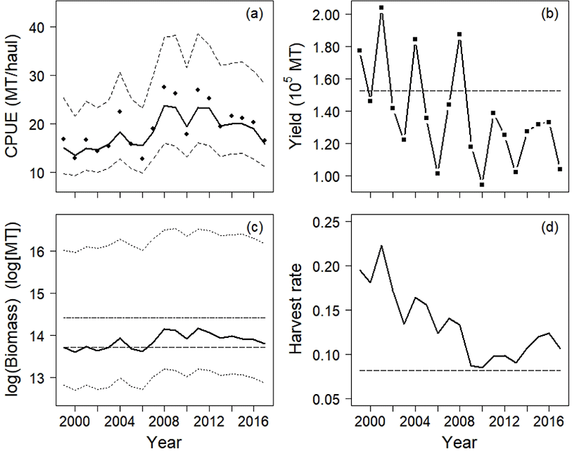
The annual biomass was below the carrying capacity, and the biomass was smaller than B_MSY in 1999, 2000, 2002, 2003, 2005, and 2006 (Fig. 4c). From 2007 onward, the predicted stock size was greater than B_MSY. The mean biomass from 1999 to 2017 was 1,064,924 MT, and the smallest and largest biomass values were 805,645 MT and 1,419,278 MT, respectively. The harvest rate, the proportion of yield to biomass, decreased during this period (Fig. 4d). The annual harvest rate remained above the calculated H_MSY.

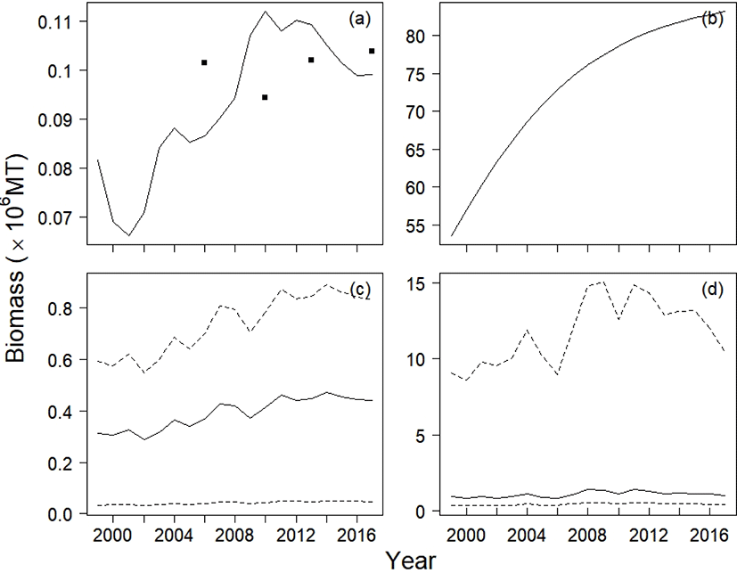
Applying the various production models, we obtained parameter estimates for each model (Table 4). The Fox and Schnute regression models gave negative estimates for carrying capacity and catchability coefficient, which are biologically absurd values. The population growth rate estimated with the Fox, YC, and Observation models war larger by about 10 to 17 times than that with the SSP model. The Schnute model interpreted the stock size as decreasing (−0.35), whereas the ASPIC program showed that the stock grew by 0.18 per year. The YC model estimated the smallest carrying capacity among the production models (160,198 MT), whereas the ASPIC program estimated the largest value (85,693,999 MT). The Observation model estimated the carrying capacity as 596,002 MT, which is about 33% of that of the SSP model. The YC model estimated the largest value for catchability coefficient (2.05 × 10⁻⁵ haul⁻¹year⁻¹), and the ASPIC program estimated the smallest value (2.59 × 10⁻⁷ haul⁻¹year⁻¹) among the production models. The Observation model estimated a catchability coefficient roughly 10 times larger than that estimated by the SSP model (4.88 × 10⁻⁵ haul⁻¹). The Observation model estimated the variance of the observation error as 0.03, roughly 42% of the corresponding SSP model estimate. All production models estimated the relative biomass in the first year, P₁₉₉₉, within the range 0.48 to 0.60. We excluded the Fox and Schnute models in comparisons of predicted CPUE and biomass trajectories because of their unreliable estimates, as evidenced by their negative values for k and q.

The predicted CPUE and biomass from the four models are listed in Figs. 5 and 6. Although all four models moderately explained the CPUE data, the residual sum of squares (RSS, equation (8) showed that the SSP outperformed the other three models in predictive accuracy (RSS_YC: 227.44, RSS_ASPIC: 280.78, RSS_Observation: 248.29, RSS_SSP: 79.91):

Fig. 5. Plots of predicted CPUE from the four production models. Black circles in all panels illustrate the annual CPUE data, and solid lines show the predicted CPUE from the four models. Panels (a–d) show the results from the Yoshimoto-Clarke model, the ASPIC program, the Observation model, and the state-space production model, respectively. Dotted lines along with the solid lines in panels (c) and (d) are 95% confidence intervals and 95% credible intervals, respectively, for predicted CPUE. CPUE, catch-per-unit-effort.

Download Original Figure

Fig. 6. Plots of predicted biomass from the four production models. The black squares in panel (a) show the yield data, and solid lines in all panels show the predicted biomass. Panels (a–d) show the results from the Yoshimoto-Clarke model, the ASPIC program, the Observation model, and the state-space production model, respectively. Dotted lines along with the solid lines in panel (c) and (d) are 95% confidence intervals and 95% credible intervals, respectively, for predicted biomass.

Download Original Figure

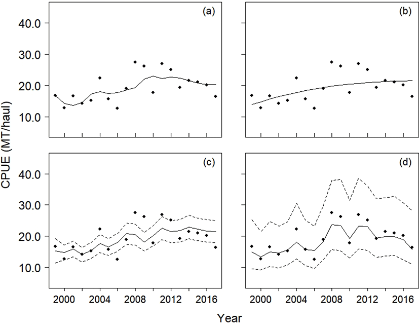
The 95% confidence intervals for the Observation model did not include the CPUE data, whereas the 95% credible intervals calculated from the SSP model did (Fig. 5c, 5d).

Although the YC model had second smallest value of RSS, it only explained the yield in years 2010 and 2013 (Fig. 6a). In the ASPIC program, the stock biomass showed monotonic increases from 1999 to 2017 (Fig. 6b), and its stock size was the largest among the four production models. The ASPIC program estimated that the average yield from 1999 to 2017 was 137,779 MT, suggesting that the stock was underexploited. The Observation model and the SSP model predicted the annual biomass to be larger than the annual yield.

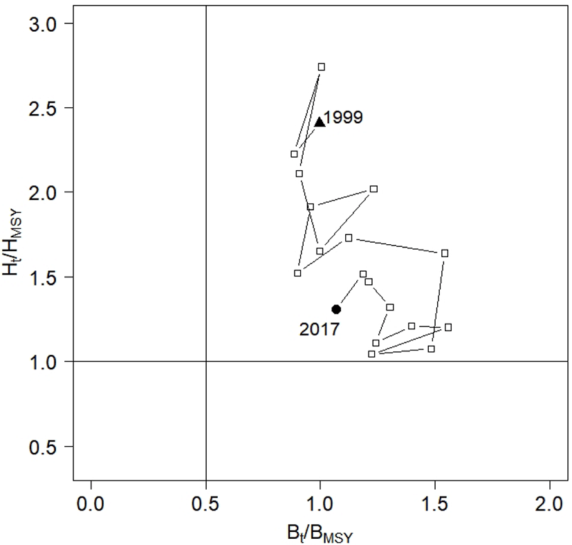
According to the National Oceanic and Atmospheric Administration (NOAA), the terms ‘overfishing’ and ‘overfished’ apply when stocks have a harvest rate larger than H_MSY (H_t > H_MSY) and the stock size is smaller than 0.5B_MSY (e.g., 0.5B_MSY > B_t). Using these definitions, we depicted the historical trajectories of the annual harvest rate and biomass in a Kobe plot (Fig. 7). The plot suggests that the stock was subject to overfishing from 1999 to 2017, and that the harvest rate exceeded H_MSY. After 1999, the annual harvest rate showed a decrease. However, the annual biomass was larger than 0.5B_MSY, indicating that the stock was not overfished during the 1999–2017 period. The graph shows a small increase in the ratio of annual biomass to B_MSY, from 1.00 in 1999 to 1.07 in 2017.

Fig. 7. Kobe plot showing the predicted trajectories of B_t / B_MSY and H_t / H_MSY from 1999 to 2017. The stock is said to be “overfished” when the biomass, B_t, is smaller than B_MSY / 2, and “overfishing” is said to occur when the harvest rate is larger than H_MSY.

Download Original Figure

Discussion

The goal of fisheries management is to maximize the profit from the catch, while also effectively conserving fish stocks (Quinn & Deriso, 1999). Estimates of growth rate and carrying capacity are directly used to calculate management policies, so estimating model parameters is crucial not only to understanding the biological properties of a population, but also to determining optimal management practices for the species.

Chub mackerel have been fished by large purse seine fisheries under quota management since 1999. In 2017, the total allowable catch (TAC) was set at 123,000 MT (Korean Ministry of Ocean and Fisheries, 2017), which was 80.56% of the MSY calculated in the present study. Hilborn (2010) introduced the concept of a ‘pretty good yield’ for managers, defined as 80% of the MSY. However, since the method of calculating TAC is not available to the public in Korea, these two values cannot be directly compared. Because the minimum legal size for chub mackerel is a total length of 21 cm, the predicted annual biomass in the present study must be interpreted as the biomass of fish larger than 21 cm. The quota in 2017 can therefore be said to be optimal only if the TAC targets the stock biomass within the legal size.

Although this study provides management principles for Korean chub mackerel, it can be dangerous to base management strategies for a species on estimates produced by a single model. We therefore strongly suggest evaluating various alternative models before setting management goals based on our results.

Compared with age-structured models, surplus production models have fewer requirements for historical data, fewer model parameters to be estimated, and simpler model structure. Setting aside these advantages, the main weakness of the present study is related to the model structure. First, because the surplus production term in the model is combined with recruitment, natural mortality, and growth, our model cannot generate separate estimates of annual recruitment and natural mortality. Therefore, age data for the stock should be collected and applied within an age-structured model, such as a statistical catch-ag-age model, not only to assess the stock year-class strength, but also for cross-validation of the estimates. Second, while chub mackerel is a highly migratory species, distributed from the East China Sea to Kurile Island (Castro Hernández and Ortega Santana, 2000; Lee & Kim, 2011; Wang et al., 2014), the model does not consider immigration or emigration. In addition to its wide range of habitats, chub mackerel is exploited by Korea, China, and Japan, in adjacent fishing grounds, which are located in the East China Sea and adjoining waters. This weakness could be addressed by aggregating annual yield and CPUE data from all three countries and applying the SSP model to assess the stock as a single population. Hiyama et al. (2002) used two data sets, one collected from Korea and one from Japan, and estimated the stock size as a single population in the East China Sea and Japan Sea based on chub mackerel migration patterns. This simple approach may provide better estimates of model parameters once rigorous studies have been conducted on the migratory pattern of the species.

State-space models, comprising process and observation equations, explicitly quantify uncertainties arising from model structure and measurement; process errors and observation errors. As mentioned above, the inclusion of process errors in our model increases the number of free parameters, such as annual biomass, and therefore necessitates additional information for parameter estimation (Prager, 1994). Carruthers et al. (2011) recommended the inclusion of prior distributions on r and k for production models, because fisheries data often contain insufficient information to obtain reliable estimates. Hilborn & Walters (1992) coined the term ‘data failure’ for instances in which the fisheries data include insufficient information about model parameters, leading to unreliable parameter estimates. For example, the negative values for carrying capacity and catchability coefficient in the Fox and Schnute model resulted from insufficient information in the data. In addition to ‘data failure’, the posteriors obtained from SSP also support this point. The posterior distributions of r and k reflected the shape of prior distributions (Fig. 2a, 2b). Posterior distributions of parameters are updated based on priors and likelihood, and the yield and CPUE data on chub mackerel did not provide sufficient information about r and k; as a result, the posteriors mirrored the corresponding priors. In practice, however, collecting data which provide sufficient information for parameter estimation is rarely possible. Therefore, the term ‘data failure’ can be translated to ‘model failure’, as models do not accurately depict biomass dynamics (Carruthers et al., 2011; Millar & Meyer, 1999; Musick & Bonfil, 2005; National Research Council, 1998; Pedersen & Berg, 2017).

While the four production models (YC, ASPIC, Observation, and SSP) fitted the CPUE data moderately well, the results showed that the SSP production model should be preferred over the others for explaining CPUE data with fluctuations. In particular, the RSSs showed that the SSP model performed best in explaining the CPUE data. While the RSS suggested that the YC model explained the CPUE data second best among the four models, the YC model failed to account for the yield in 2010 and 2013. The ASPIC program indicated that the stock was severely underexploited throughout the whole duration of the study. To be specific, the mean ratio of the B_t to B_MSY was 1.6, and the mean ratio of F_t to F_MSY (fishing mortality rate that corresponds to MSY) was 0.02. The ASPIC program may therefore provide an optimistic view of chub mackerel stock, which allows fishermen to exploit the stock more extensively than does the present level. The Observation model provided uncertainties for the predicted CPUE, as did the SSP model. However, the intervals of the model were too narrow to include the CPUE data (Fig. 5c), which, could be addressed by the SSP model (Fig. 5d). The Observation model therefore may consider the observation errors only, whereas the SSP model incorporated both process and observation errors, resulting in wider credible intervals for the predicted CPUE. In short, a SSP model can be a solution for CPUE data with fluctuations.

Priors were a key factor in the implementation of the SSP model. In practice, we used the mode and CV to determine hyperparameters for each model parameter, and then obtained prior distributions through trial and error, to stabilize the numerical optimization. As the priors contain information on parameters, biologically absurd priors were excluded. For example, positive values were chosen for the modes of growth rate r, catchability coefficient q, and P₁₉₉₉. The mode for carrying capacity, k, was only selected when its value was larger than the largest yield. To address our uncertainty regarding priors, we set the CV to be larger than 50% for each parameter. The posterior distributions obtained with the priors and likelihood function in the present study can be used as priors in future studies on Korean chub mackerel. The script software ADMB-RE performed both numerical optimization and MCMC sampling. Although we selected priors that assisted in the numerical optimization of the likelihood function, it is also possible to obtain posterior distributions through the script software without editing its code. Therefore, we recommend taking advantage of this powerful statistical tool for the implementation of Bayesian state-space models.

Conclusions

This study aimed to fit CPUE data with fluctuations, and to assess Korean chub mackerel stock. We applied a SSP model to the annual yield and CPUE data collected from 1999 to 2017, with prior distributions for the model parameters (r, k, q, ${\sigma }_p^2$, ${\sigma }_o^2$, P₁₉₉₉), using the software ADMB-RE. We estimated model parameters including intrinsic growth rate r, carrying capacity k, and annual biomass, and provided management references (MSY, B_MSY, and H_MSY). We concluded that Korean chub mackerel stock have been subjected to overfishing, but were not overfished during 1999–2017, based on the trajectories of H_t / H_MSY, and B_t / B_MSY. The findings of this study suggest that practitioners should choose a SSP model which considers two sources of variability, and to fit the CPUE data with fluctuations. Further studies into the migration patterns of chub mackerel must be carried out in order to assess the stock as a single population fished in the East China Sea.