Background
Based on the statistical sampling theory, most developed countries in fisheries management have deployed a bottom trawl survey on a periodic basis (e.g., seasonally) for several decades as part of groundfish stock assessments (NEFSC 2012; NWFSC 2011). They use the survey data to calculate the relative size of a fish population, called “the survey index” of a fish stock (Hyun et al. 2015; NEFSC 2012). They commonly used the stratified random sampling, considered to be appropriate for a survey over a large area such as ocean areas or lakes (Hyun et al. 2015; Smith and Gavaris 1993; Smith and Hubley 2014). For example, the bottom trawl survey of the US west and east coast groundfish and a count survey in Columbia River salmon spawning areas in the Northwestern USA have been based on a stratified random sampling design (Hyun et al. 2015; NEFSC 2012; NWFSC 2011).
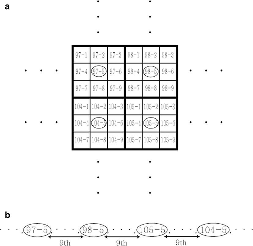
On the other hand, South Korea’s (hereafter, Korea) stock assessments have a relatively short history. The Korean National Institute of Fisheries Science (KNIFS) started a bottom trawl survey about one decade ago (Lee 2018; Lee and Hyun 2017). Unlike the common practice of stratified random sampling, KNIFS has sampled groundfish on a regular basis every spring and fall. Rectangular grids were set over the ocean around the Korean peninsula, whose sides are one-half degree of latitude by one-half degree of longitude (Fig. 1), and KNIFS had sampled once per grid square in each survey season (see the “Methods” section for details). Such survey data have been accumulated but rarely used for inferring the survey indices of groundfish stocks, and one of our objectives in this paper is to illustrate how to use those data for estimating the survey indices of fish stocks and quantifying the uncertainty of the estimated survey indices. We would like to underscore that our analysis of the survey data is conditional on the data collection. In other words, we have nothing to do with the initial stage of the sampling, which is to “design” a survey. Thus, this paper’s issues do not include which sampling design is more or less appropriate.

For the regularity, we suggest that the systematic sampling theory should be applied for estimating the survey index and its uncertainty. In this paper, we intend to illustrate how to apply the systematic sampling theory to the Korean bottom trawl survey data, especially how to quantify uncertainty of the survey index of a fish stock under the systematic sampling method.
Methods
The bottom trawl survey has been deployed every spring and fall since 2000, and it has trawled once per grid cell (Fig. 1) within each survey season. Each grid cell is a rectangle whose sides are one-half degree of latitude by one-half degree of longitude and which is divided into nine nested grid cells (Fig. 1). Generally, the survey has trawled at the center nested grid cell (“-5” in Figs. 1 and 2) unless the survey had a problem (e.g., running into a rocky bottom). The practice of trawling once per grid cell (i.e., at the center nested grid cell) indicates an implicit assumption that the fish density is equal across all nine nested grid cells within a grid cell. However, not all grid cells have the same area, so we needed to treat grid cells separately, e.g., we calculated the area of each grid cell when calculating the survey index (i.e., the relative size of a fish population). We calculated the area of each grid cell, using the area by latitude and longitude, and showed them in Appendix Table 4.

In the systematic sampling, every kth item is inspected, and such a sample is called a 1-in-k systematic sample (Scheaffer et al. 2012). From this perspective, those nested grids selected for the bottom trawl survey can be treated as a 1-in-9 systematic sample, because every ninth item is inspected (Fig. 2b). For the scheme, the sampling unit, ysi, is the survey catch of stock s in number or weight caught by a standard tow in the center nested grid in grid cell i.
If the average of the sample units of stock s collected by all survey tows (i.e., ) is multiplied by the total number of possible tows in the population area, then the resultant quantity indicates the relative size of the stock’s population, also called the survey index of stock s (NEFSC 2012): , where N is the total number of possible tows in the population area, which is calculated by dividing the area of grid cell i by the area covered by a standard tow (Smith and Lundy 2006). In our case, it should be the weighted average of the area of grid cell i divided by the area covered by a standard tow:
See Table 1 for notations. However, the reason the survey index indicates the relative size of a fish population is due to unknown catchability or vulnerability, which is different by species, area, and time (e.g., season) (NEFSC 2012). For this reason, the survey index means the “minimum swept area abundance (or biomass)” (NEFSC 2012).
Notation | Description |
|---|---|
i | Grid cell. Each grid cell is divided into nine nested grids. See Fig. 1 for the location of grid cell i. |
s | Fish stock |
ai | The swept (trawled) area in grid cell i |
Ti | The area of grid cell i. See Appendix Table 4 for the area of grid cell i. |
ysi | Number (or weight) of fish stock s, caught by a standard trawl in one of the nine nested grids in grid cell i. This quantity is defined as the sampling unit. |
N | The total number of possible tows in the population area. |
Ys | The survey index (in number) of a fish stock s. |
Bs | The survey index (in weight) of a fish stock s. |
dsi | Differences between successive sampling units, i.e., dsi = ys, i + 1 − ysi. |
n | The number of the entire tows, which is the sample size. |
^ | In this paper, the hat notation is the expected value of a random variable, e.g., E{Ys} |
Although the bottom trawl survey did not deploy a simple random sampling (SRS) (see the “Background” section), we applied SRS to the survey data as the reference, which is to be compared with results from the systematic sampling (SYS) below. Under SRS and SYS, we show the expected value of the survey index and its uncertainty. When denoting the expected value of a random variable as its hat (^) in this paper (e.g., ),
Then, it is easy to derive the variance of by applying the central limit theorem (CLT) (Casella and Berger 1990) to , i.e.,
where Var{ys} is the sample variance of ysis (i.e., Var{ys} = ) and the term is the finite population correction (FPC) (Cochran 1977; Scheaffer et al. 2012). Finally, the variance of the survey index is:
Equations 2 and 4 are the expected value of the survey index and its uncertainty under SRS (Cochran 1977; Scheaffer et al. 2012). The expected value of the survey index under SYS is the same as that under SRS, but its variance under SYS is different from that under SRS. When following Scheaffer et al. (2012) for the variance calculation under SYS, we needed to arrange the sampling units in temporal order (e.g., ys1, ys2, ⋯, ysn), select two sample units ysi and ys, i + 1, and then construct dsi = ys, i + 1 − ysi. Under this scheme, it is straightforward that E{dsi} = 0 and Var{dsi} = Var{ys, i + 1 − ysi} = 2 Var{ys} with the assumption that the variances of the sampling units are constant across grid cells and the sampling units are independent (i.e., Cov{ys, i + 1, ysi} = 0). On the other hand, Var{dsi} = . In Scheaffer et al. (2012), Var{dsi} is expressed as the maximum likelihood estimator, i.e., Var{dsi} = ; note that the denominator of (n − 1) is the number of dsis (see page 238 in Scheaffer et al. (2012)). However, we used Var{dsi} as the unbiased estimator in this paper, where the denominator is (n − 2) by subtracting 1 from the number of dsis (i.e.,. (n − 1 − 1)). Therefore,
We use the mean of the sampling unit, , to calculate the variance of . By CLT, Var{} is:
where the term is FPC (Cochran 1977; Scheaffer et al. 2012). To contrast the variance of under SYS (Eq. 6) with that under SRS (Eq. 3), we put subscript “SYS” in Eq. 6. Therefore, we can calculate Var{} under SYS by replacing Var{} in Eq. 4 by in Eq. 6.In summary, the expected value of the survey index, , is Eq. 2 regardless of whether assuming SRS or SYS as the sampling design. However, Var{} used for calculating Var{} (Eq. 4) is given by Eq. 3 if we assume SRS, while that is Eq. 6 if assuming SYS.
Results and discussion
The point estimate of the survey index of a fish stock remains the same regardless of applying SRS or SYS, and thus, the major issue lies in the precision of the survey index between SRS and SYS. Overall, the survey index under SYS was more precise than that under SRS. In estimates of the survey index in number (), those estimates for 10 of the 11 stocks were more precise under SYS than those under SRS during both the spring and fall surveys (Table 2). In estimates of the survey index in biomass (), a similar pattern was found, where those estimates for 9 of the 11 stocks were more precise under SYS than those under SRS during the spring survey while those for 10 stocks were more precise under SYS than those under SRS during the fall survey (Table 3). For example, the standard error of for stock 10 (black scraper) under SYS was reduced by 28.76% from that under SRS in the spring survey while that for stock 1 (Pacific cod) under SYS decreased by 26.70% from that under SRS in the fall survey (Table 2). In case of the standard error of , that for stock 2 (White croaker/Silver jewfish) was 30.65% lower in the spring survey while that for stock 1 (Pacific cod) was 31.13% lower in the fall survey (Table 3).
The column of “Change (%)” indicates a change in the standard error (SE) under the systematic sampling (SYS) relative to that under the simple random sampling (SRS), i.e., Change (%) = . Those 11 stocks are as follows: 1 = Pacific cod (Gadus macrocephalus); 2 = White croaker/Silver jewfish (Argyrosomus argentatus); 3 = Pacific herring (Clupea pallasii); 4 = Red tilefish (Branchiostegus japonicus); 5 = Blackfin flounder (Glyptocephalus stelleri); 6 = Yellow croaker (Larimichthys polyactis); 7 = Gazami crab (Portunus trituberculatus); 8 = Mottled skate (Raja pulchra); 9 = Chub mackerel (Scomber japonicus); 10 = Black scraper (Thamnaconus modestus); 11 = Largehead hairtail (Trichiurus lepturus)
The column of “Change (%)” indicates a change in the standard error (SE) under the systematic sampling (SYS) relative to that under the simple random sampling (SRS), i.e., Change (%) = . Those 11 stocks are as follows: 1 = Pacific cod (Gadus macrocephalus); 2 = White croaker/Silver jewfish (Argyrosomus argentatus); 3 = Pacific herring (Clupea pallasii); 4 = Red tilefish (Branchiostegus japonicus); 5 = Blackfin flounder (Glyptocephalus stelleri); 6 = Yellow croaker (Larimichthys polyactis); 7 = Gazami crab (Portunus trituberculatus); 8 = Mottled skate (Raja pulchra); 9 = Chub mackerel (Scomber japonicus); 10 = Black scraper (Thamnaconus modestus); 11 = Largehead hairtail (Trichiurus lepturus)
In the opposite cases where the standard error of the survey index under SYS was larger than that under SRS, those differences in the standard error were negligible and such cases were few: see Table 2 for change (%) of 1.50 and 1.81% in for only stock 3 (Pacific herring) during both the spring and fall surveys, and Table 3 for change (%) of 1.50~1.75% in for stock 3 (Pacific herring) and 4 (Redtile fish) during the spring survey, and change (%) of 1.66% for only stock 3 during the fall survey. In other words, in the few cases that they were observed, the increase was at most 1.75%.
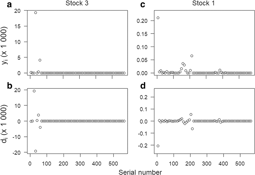
It was not difficult to figure out why such a negligible increase could happen in the standard errors of the survey index of a few stocks when changing the assumption from SRS to SYS. Such a case could happen when one or another of the sampling units (i.e., ysis) is extremely different from the majority, e.g., most of the sampling units of stock 3 collected during the fall survey were less than 1000 but the fourth sampling unit (serial number 32) was 19,292 (Fig. 3a). The resultant differences between successive sampling units (i.e., dsis) included this substantial variability, e.g., note the third and fourth successive sampling units were ±19,292 (see ds3 and ds4 in Fig. 3b). For the contrast, the usual case is shown in Fig. 3c, d. The sampling units of stock 1 caught during the fall survey ranged from 0 to 210 (Fig. 3c), which were much narrower than Fig. 1a. The range of the resultant dsis became further narrower, at most 206 (i.e., the absolute value of − 206 in Fig. 3d).

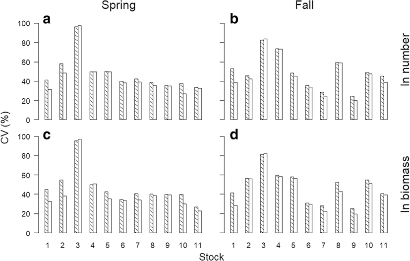
Differences in the coefficient of variation (CV) of the survey index of a fish stock between SRS and SYS methods were not interesting because of those in the standard errors between them. However, it is worth noting the wide range of CVs of the survey indices among stocks (Fig. 4). CVs of the survey indices in number ranged from 24.5 to 96.2% under SRS while those ranged from 20.1 to 97.6% under SYS (Fig. 4a, b). Those in biomass ranged 25.1 to 95.5% under SRS while those ranged from 19.4 to 96.9% under SYS (Fig. 4c, d). Under SRS, the survey index of stock 3 (Pacific herring) was most uncertain while that of stock 9 (Chub mackerel) was least uncertain (shaded bars in Fig. 4). Under SYS, the survey indices of stock 3 and stock 9 were also most uncertain and least uncertain, respectively (blank bars in Fig. 4). Such a wide range in CVs of the survey indices implies that a much more sample size than those used in 2014 (n = 67 in the spring survey, and n = 64 in the fall survey) would be needed to reduce such a large uncertainty. If hypothetically setting CV to 40% were considered satisfactory, then CVs of the survey indices of only three stocks (stock 1, 6, and 9) were commonly below 40% even under SYS (blank bars in Fig. 4).

One of the common issues in fish stock assessments lies in whether to express the population size as abundance or biomass. Although our paper focuses on the methodology about the systematic sampling, a practical management issue could be which one between the survey index in number or weight to be used. Especially in the situation that fish ages in survey catches were not determined, the survey index in weight must be preferred to that in number because the latter could include juvenile fish, whose body sizes are too small to be considered to be a spawning stock and to be worthy of a commercial fishery.
To our knowledge, our paper is the first to formally show how to apply the SYS theory to the actual data collected by the Korean bottom trawl surveys. For estimation of the survey index of a fish stock and its uncertainty, Lee and Hyun (2017) applied the method of the stratified random sampling to those data, arbitrarily assuming three strata (east, south, and west), as well as applied the SRS method. The arbitrary assumption was motivated to convince Korean managers that the stratified random sampling outperformed SRS especially in estimating the precision of the survey indices. As we described in the “Background” section, the current practice of the bottom trawl survey started about one decade ago where groundfish were sampled once per grid cell (Fig. 1). Although we think KNIFS should consider changing the status quo to stratified random samplings, this paper confirms that the current SYS outperforms SRS, and it is worth using, until KNIFS eventually figures out appropriate strata into which the population area should be divided.
Conclusions
We applied the SYS and SRS methods to data collected by the bottom trawl surveys during spring and fall in 2014 to infer the survey indices of 11 Korean groundfish stocks. Overall, the survey indices estimated under SYS were more precise than those estimated under SRS. Such results are consistent with the statistical sampling theories with respect to SYS and SRS. The inference of the survey indices of fish stocks is a necessary part of stock assessments, with which the commercial fishery catch data must be integrated for inferring the fish population sizes and other associated parameters (e.g., fishing mortality and overfishing limits). We suggest KNIFS should apply the SYS methods illustrated in this paper to infer the survey indices of Korean groundfish stocks. However, we recommend that KNIFS should eventually change the sampling design to stratified random samplings.


