Oceanographic indicators for the occurrence of anchovy eggs inferred from generalized additive models

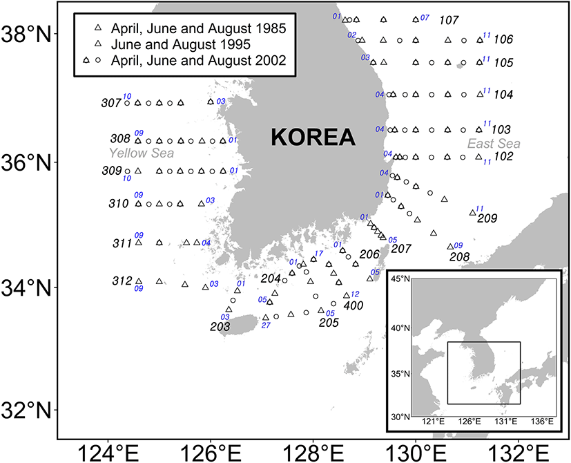
To determine the seasonal factors influencing anchovy spawning grounds, we used ichthyoplankton data collected from a zooplankton net (45 cm mouth diameter, 0.333 mm mesh size) during the oceanic survey regularly conducted by National Institute of Fisheries Science (NIFS). A total of 492 samples were collected along 19 lines in the East, West, and South Seas during April, June, and August of 1985 and 2002, and in June and August of 1995 (Fig. 1). Oceanographic data (seawater temperature, salinity, and dissolved oxygen (DO); at depths of 10 m and 50 m), coinciding with the same time period as the NIFS surveys, were retrieved from the Korea Oceanographic Data Center (KODC). As anchovy eggs are distributed mostly at the 10–50 m water layer (Kim and Choi 1988; Boyra et al. 2003), we used the differences in temperature, salinity, and DO at 10 m and 50 m water layers as the levels of indication of vertical mixing in the ocean.

Fig. 1. Typical stations for the sampling of anchovy eggs and zooplankton, and oceanography observations in Korean waters during 1985, 1995, and 2002

Download Original Figure

Egg density was calculated as the number of eggs per m² of sea surface area. Zooplankton biomass (mg/m³) was estimated from the wet weight of each sample after removing the eggs. We used the egg distribution pattern to indicate the extent of the anchovy spawning ground, which was explained using a confocal ellipse of the distribution area and the density (D) at each station, and was calculated as follows:

where X and Y are the longitude and latitude of the station (i), and the X and Y bars are the confocal of the ellipses. The ellipses can be described by two principle axes of the fishing grounds: the major axis (b1) and the minor axis (b2), which are at right angles to each other. The slopes of b1 and b2 were calculated from the covariance of the longitude (X) and latitude (Y) of the station, weighted by the density (D), as estimated from the survey (Sokal and Rohlf 1995; Kim et al. 2005).

Based on the oceanographic data system by the KODC, the total survey area was divided into three distinct areas: the East Sea (lines 102–106, 208–209), the South Sea (lines 203–207), and the West Sea (lines 307–312) of Korea. Box plots and descriptive statistics (mean and variance) were used to summarize the distribution of egg density and the oceanographic factors for the total monitoring period (total egg density) by year, month, and area. We applied statistical methods with the ordinated seven variables: temperature, salinity, and DO at the 10 m depth layer, the differences between the 10 m and 50 m depth layers for temperature, salinity, and DO and zooplankton abundance. To determine differences in egg density, we analyzed egg density over the years and survey lines during April, and among years, months, and regions during June and August using a multi-factor analysis of variance (MANOVA). Egg density data collected during June and August were combined for subsequent analysis as the MANOVA showed no significant differences between the densities in these 2 months.

We applied regular GAMs for the total and spring seasons (April) and for the data in each area during the summer season (June and August) to explain the occurrence of anchovy spawning grounds based on oceanographic factors and compared the results of the models. Since egg density is characterized by high variability due to drift and high embryonic mortality, we used two spatial strata and quantile GAMs to determine the indicators of the spawning grounds based on the absence/presence of eggs, the log-transformed egg density, and high density (above 70–90% quantiles) for the total data. For the first stratum (with egg presence as a response variable), GAMs were constructed using a binomial error structure and a logit-link function with an unbiased risk estimator (UBRE). For the second stratum, GAMs with log-transformed egg density as a response variable and oceanic factors as explanatory variables were built assuming a Gaussian error structure and an identity-link function with the generalized cross validation (GCV). Quantile generalized additive models were used to estimate either the conditional median or other quantiles of the response variables based on Elf with restricted maximum likelihood (REML) criterion. The upper boundary describes how abundance is limited by this factor, while the variation below the upper boundary reflects the limiting effect on the abundance of environmental attributes other than the factor of interest (Vaz et al. 2008). We assumed that a high density of eggs indicates the center of spawning and the eggs spread out gradually as they developed. To confirm the effect of the oceanic factors on the egg density, confidence intervals around the predicted 0.10th and 0.90th quantiles in the quantile GAM were used to model the τth quantile (where τ ∈ (0,1)) of the response (y), and conditional on a p-dimensional vector of covariates (x). We fitted variables as a smooth term at the 0.10th, 0.50th, and 0.90th quantile of residual-abundance for total data and the 0.50th, 0.70th, 0.80th, and 0.90th quantile of residual-abundance for spring because of the seasonal changes in the ratio of absence stations: absence was far more frequent in spring and could overwhelm the shape of abundance distributions.

We applied the PCA and GAMs with the seven ordinated variables: temperature, salinity, and DO at the 10 m depth layer, and the difference between the 10 m and 50 m depth layers for temperature, salinity, and DO in addition to the zooplankton abundances based on the correlations. The PCA can be used to eliminate redundant information by removing correlated features in the predictor variables, and then using that to create new independent variables (Li et al. 2017; Liu et al. 2019). In our study, we used the PCA to simplify our models and eliminate multi-collinearity among oceanographic variables. The PCA-based GAMs were used to reduce variables, and smoothing functions were used on the predicted principal components (PCs). Independent variables were selected based on the environmental conditions and PCs were selected from the results of the PCA.

In this study, the general form of the GAM is explained by the following equation:

where E[y] is the expected value of the response (dependent) variable y, a is the intercept of the parametric term which represents the mean of the response variable, s is the smoothing function based on the thin plate regression spline, Vi represents the independent variables, and ε is the error term. We restricted the number of degrees of freedom (df = 4, k = 3) to minimize model over-fitting.

The initial models of the GAM contained all covariates and were optimized with backward selection based on a reduction in Akaike’s information criterion (AIC). We selected the best models based on the gain in deviance explained (% Dev) relative to the basic model, whilst minimizing the AIC, GCV, UBRE, and REML criteria. To avoid overfitting and to reduce collinearity, all covariates were examined using Pearson’s rank correlations to identify variables with low correlation values (Pearson correlation r < 0.6) in the modeling process. Multi-collinearity among the predictor variables was assessed by calculating the variance inflation factor (VIF) using a cutoff value of 5 with the function (Liu et al. 2019; Hoeffle et al. 2014). The GAMs and QGAMs were fitted using the “mgcv” (Wood 2019) and “qgam” (Fasiolo et al. 2020) in R-3.4.2.

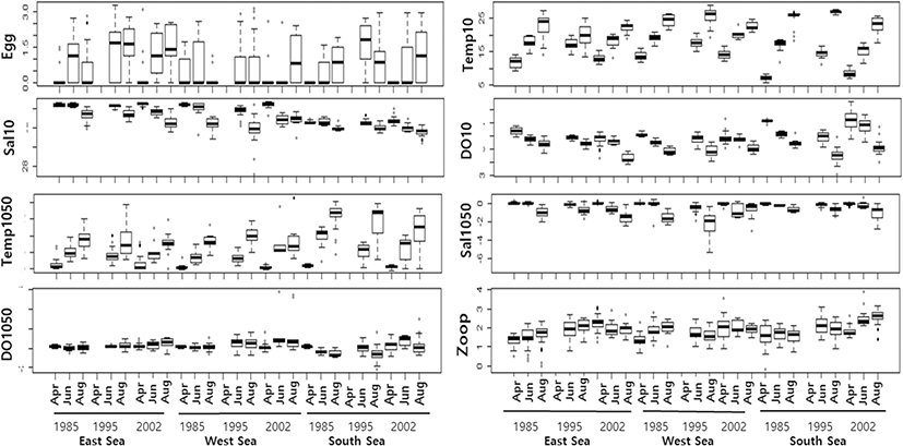
Descriptive statistics were used to summarize the distribution of egg density and oceanographic factors (Table 1 and Fig. 2). Egg density and oceanographic factors varied widely and were highly skewed with a high level of kurtosis. Egg density was lowest in April and highest in June and August, with particularly high densities observed in the East and South Seas during 1995, and in the West Sea during August 2002. In all areas, the oceanographic parameters (measured at depths of 10 m) varied seasonally, with trends of increasing temperature and decreasing salinity and DO from April to August. Concurrently, the temperature difference between the 10 m and 50 m depth layers decreased, while the salinity difference increased from April to August. The DO difference between 10 m and 50 m varied widely during June and August. Zooplankton density increased from April to June and was particularly high during 1995 and 2002 in the East Sea and during 2002 in the South Sea (Fig. 2).

Fig. 2. Boxplots of anchovy egg density (egg; Log₁₀ no./m²), zooplankton biomass (Zoop; Log₁₀ mg/m³) and oceanographic factors with the median and standard deviation. Temperature (Temp10; °C), salinity (Sal10; psu) and DO (DO10; ml/L) were measured at the 10 m depth layer. Temperature difference (Temp1050; °C), salinity difference (Sal1050; psu), and DO difference (DO1050; ml/L) between 10 m and 50 m depth

Download Original Figure

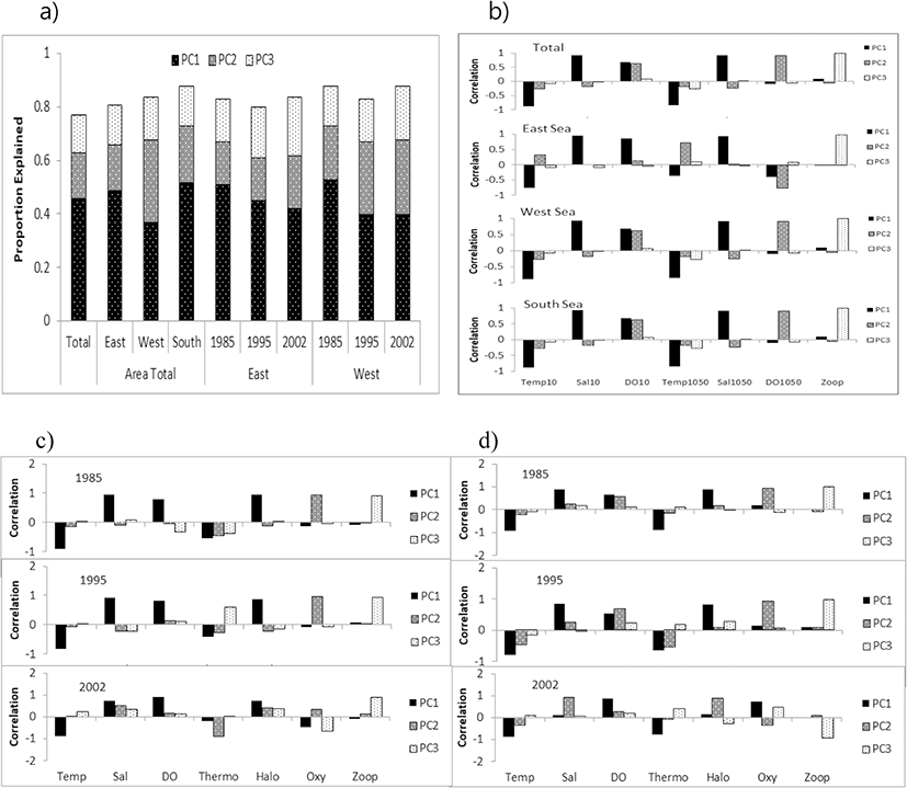
The results from the PCA revealed an optimal subset of explanatory variables, which represented a cumulative 77–88% of the total variance across three components (Fig. 3a). Temperature, salinity and DO at 10 m depth and the value of the difference between 10 and 50 m were mostly related to the first component (PC1) and represented 37–53% of the variance; DO and the DO difference between 10 m and 50 m were mostly related to the second component (PC2) and represented 16–31% of the variance; and zooplankton density was related to the third component (PC3) and represented 14–20% of the variance, with correlation values varying among the area and the year (Fig. 3a, b–d).

Fig. 3. The results of PCA of the seven oceanographic factors: temperature (Temp10, °C), salinity (Sal10, psu) and DO (dissolved oxygen; DO10, ml/L) as measured at a depth of 10 m; and the mixing index of temperature (Temp1050, °C), salinity (Sal1050, psu), and DO (dissolved oxygen; DO1050, ml/L) for the difference between 10 m and 50 m depth layer (Sal1050, psu), and zooplankton biomass (Zoop, Log₁₀ mg/m³); in the East, West, and South Seas of Korea during April of 1985 and 2002, and June and August of 1985, 1995, and 2002. Proportion of explained variances for the 3 components (a), correlation for the variables in total (b), East Sea (c), and West Sea (d) during summer in 1985, 1995, and 2002

Download Original Figure

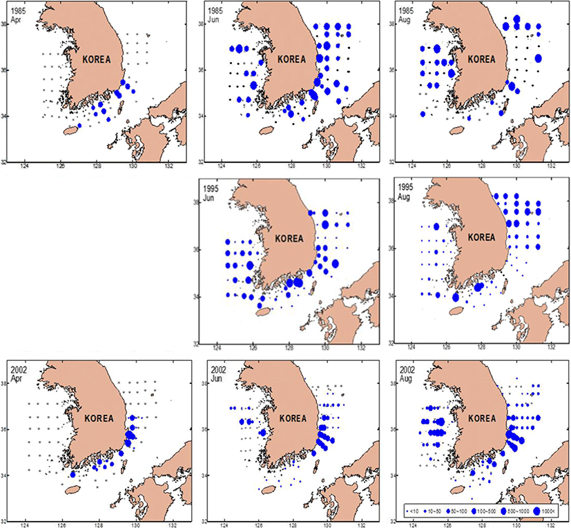
Based on measurements from 1985, 1995, and 2002, the monthly changes in the anchovy spawning grounds were characterized by seasonal variations in the density of anchovy eggs (Fig. 4). In April, the egg distribution was limited to the South Sea and the southern East Sea, whereas by June and August, eggs were widely distributed in the mid-East and West Seas. In April 1985, anchovy eggs were present at low densities (< 50 ind./m²) in the South Sea and in the southern East Sea. However, by April 2002, the egg distribution changed from the southern East Sea and southern coast of the mid-East Sea (P = 0.041, with a significant difference in densities at the survey line between April 1985 and 2002). In June 1985 and 1995, the eggs were distributed over wide areas of Korean waters. In August, the eggs were concentrated in the mid-East Sea and occurred along coastal areas of the mid and southern West Sea and the East Sea (> 500 ind./m²). In June 2002, the eggs were found at high densities in the waters of the mid-West and southern East Seas. In August 2002, the distribution of eggs was concentrated offshore of the West Sea (> 1000 ind./m²) and in coastal areas of the southern East Sea. Results of the MANOVA analysis of egg density during summer (June and August) showed significant differences by year (P = 0.002) and area (P = 0.017).

Fig. 4. Spatial distribution (blue circle) of anchovy eggs and sampling stations (dot) in Korean waters during April in 1985 and 2002, and June and August in 1985, 1995, and 2002 (unit of egg density in the legend: Ind.No/m²)

Download Original Figure

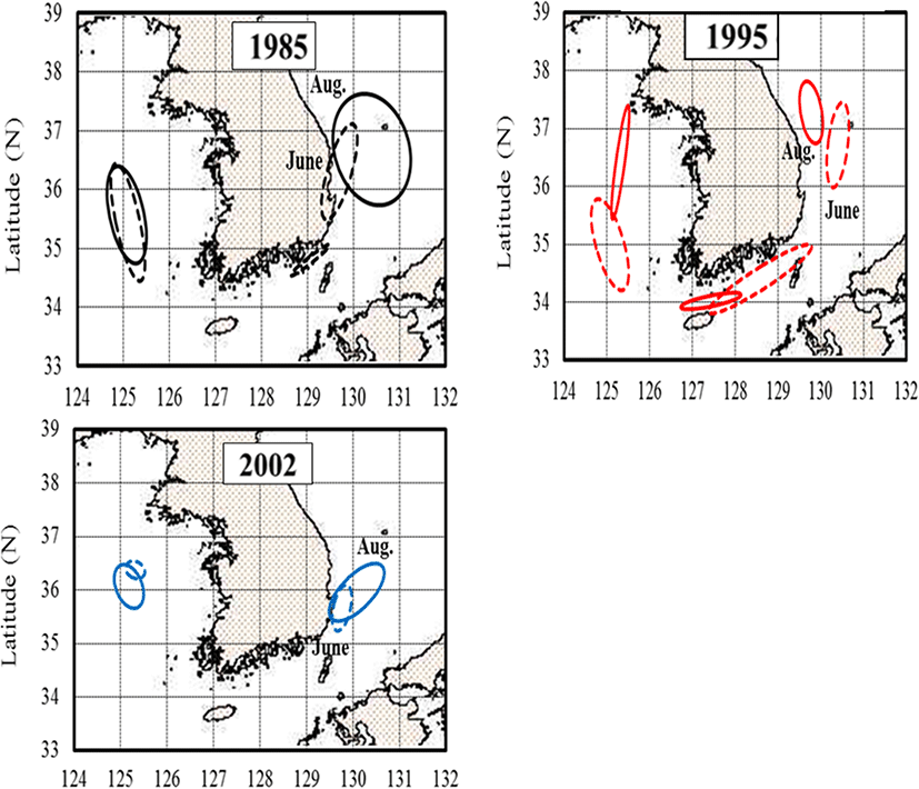
The distribution of anchovy eggs explained using confocal ellipses with axes and slopes are shown in Fig. 5. The joint confidence regions were compared with the egg densities in each month between 1985, 1995, and 2002. Based on Fig. 5, it is apparent that their spawning ground was distributed in the East Sea in 2002 compared to 1985 and 1995, while their spawning ground changed northward in the West Sea in 1995 in comparison to 1985 and 2002.

Fig. 5. Distribution of anchovy eggs explained using confocal ellipses of distribution areas, weighted by the density at each station, in Korean waters during June (dashed-line) and August (solod line) in 1985, 1995, and 2002

Download Original Figure

The results of the regular (binomial and Gaussian) GAMs and QGAMs (Elf) revealed that various environmental factors at the 10 m depth layer and the values of difference between the 10 and 50 m depth layer had significant effects on egg density (Tables 2, 3, and 4). The shapes of the functional forms for the covariates are illustrated in Figs. 6, 7, and 8, where the solid lines represent the main effect of the independent variables and the dotted lines represent 95 % confidence intervals. The observed waves indicated that egg densities had non-linear responses to the covariates. Total egg density was non-linearly related to temperature, salinity, and DO at a depth of 10 m, the salinity difference between 10 m and 50 m, and log-transformed zooplankton density in the Gaussian error structure (Table 2, Fig. 6a). There was no significant effect of zooplankton density on egg presence based on results from the GAM with a binomial distribution. In addition, egg density was not significantly affected by DO (Table 2). Although the probability of egg presence was nearly maintained at a temperature of 10 m (Fig. 6b, 0.10th, and 0.50th quantiles), egg density probability peaked at 18–20 °C (Fig. 6a, b, 0.90th quantile) and especially increased in the presence of high zooplankton density in the upper 0.90th quantiles of egg density (Fig. 6b). Environmental variables explained 12.4% (binomial), 13.0% (Gaussian), and 17.7% (Elf) of the density of eggs, respectively (Table 2).

Fig. 6. Results of the regular GAMs (a) and QGAMs (b) for the total egg data, and the regular GAMs (c) and QGAMs (d) for seasonal data of the spring (April) assuming a Gaussian and ELF error distribution; temperature (Temp10, °C), salinity (Sal10,psu), and dissolved oxygen (DO10, ml/L) at the 10 m depth layer, the salinity difference between 10 m and 50 m depth layer (Sal1050, psu), and zooplankton biomass (Zoop, Log₁₀ mg/m³). The solid lines represent the main effects of the independent variables. The dotted lines represent the 95% confidence intervals in the GAMs (a and c). Each legend (b and d) represents the quantiles (0.1th, 0.5th, 0.7th, 0.9th) of the egg density

Download Original Figure

Fig 7. Results of the regular GAMs for the seasonal data during summer (June and August) assuming a Gaussian error distribution; East Sea in 1985 (a), 1995 (b), 2002 (c), and West Sea in 1985 (d), 1995 (e), 2002 (f), South Sea in 1985 (g), and 1995 (h); temperature (Temp10, °C), salinity (Sal10, psu), and DO (DO10, ml/L) at the 10-m depth layer and zooplankton biomass (Zoop, Log₁₀ mg/m³). The difference between 10 m and 50 m depth layer on the temperature (Temp1050, °C), salinity (Sal1050, psu), DO (DO1050, ml/L) are represented as the mixing index in the ocean. The solid lines represent the main effects of the independent variables. The dotted lines represent the 95 % confidence intervals

Download Original Figure

Fig. 8. Results of the PCA-based GAM assuming a Gaussian error distribution, for the total egg data during June and August, 1985, 1995, and 2002 in the East Sea (a) and West Sea (b). Composition of PC1, PC2, and PC3 are represented from Fig. 3. The solid lines represent the main effects of the independent variables. The dotted lines represent the 95% confidence intervals

Download Original Figure

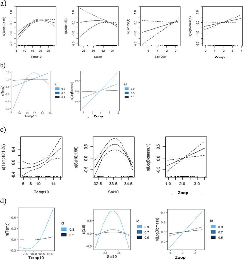
The shape of the functional forms during spring (April) indicated that egg density had a significant positive relationship with temperature (Fig. 6c), and a dome-type relationship with salinity in the upper 0.80th and 0.90th quantiles of egg density, which peaked with salinity over 33.5 psu (Fig. 6d). This explained 16.8–48.0% of the deviance in 1985 and 2002 (Table 2).

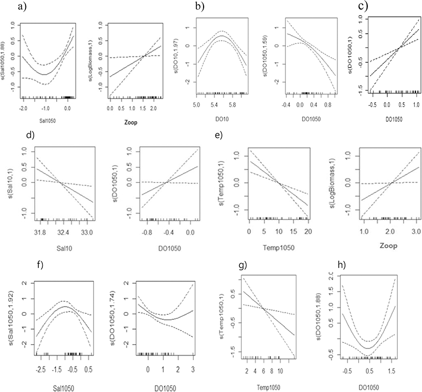
Egg density during the summer (June and August) was mostly found to be non-linearly related to parameters in the Gaussian error structure, with steep increasing or decreasing trends in the upper 0.50th–0.90th quantiles (Fig. 7). Egg density in the East Sea was significantly related to the halocline index in conversely dome-type, and with zooplankton density in a positive linear shape during 1985 (Fig. 7a); with DO in a dome-type and oxy-cline index in an inversely linear shape in 1995 (Fig. 7b); with the DO difference between the 10 and 50 m layer linearly during 2002 (Fig. 7c), with 29.9–41.1% and 39.1–63.2% of the deviance explained in the GAM and QGAM, respectively (Table 3). Egg density in the West Sea had a negative relationship with salinity and a positive relationship with the DO difference between the 10 and 50 m layer in 1985 (Fig. 7d), and exhibited a negative relationship with the temperature difference between the 10 and 50 m layer and a positive relationship with zooplankton density in 1995 (Fig. 7e). It was also related to dome-type relationship with the salinity difference between the 10 and 50 m layer and a converse dome-shape with the DO difference between the 10 and 50 m layer in 2002 (Fig. 7f), with 18.5–41.6% and 38.6–56.3% of the deviance explained by the GAM and the QGAM, respectively (Table 3). Egg density in the South Sea had a significant negative relationship with the temperature difference between the 10 m and 50 m layer in 1985, and a dome-shaped relationship with the salinity difference between the 10 m and 50 m layer in 1995 (Fig. 7h), with 14.3–24.1% and 14.3–38.3% of the deviance explained in the GAM and the QGAM, respectively (Table 3).

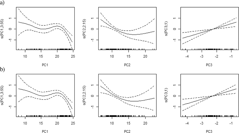
In the PCA-based GAM, the variance explained by the final regression model was 33.2–67.0% for egg density in the East Sea and 27.3–64.3% for density in the West Sea, which were higher than the values of the results obtained by the regular GAM and QGAM. Egg densities in the East Sea and West Sea exhibited similar effects of non-linear decrease for PC1 and increasing effects for PC3, but had different effects for PC2, with a conversely dome-shape in the East Sea and a positive relationship in the West Sea. The yearly egg density had a significant relationship with PC1, PC2, and PC3 in the East Sea, but not in the West Sea (Table 4, Fig. 8).

Many studies have been conducted to investigate the factors affecting the distribution of anchovy eggs in Korean coastal waters; these have shown that anchovy eggs are distributed over a wide range, and their distribution shows a high skewness and kurtosis (Lim and Ok 1977; Kim 1983; Table 1 and Fig. 2). Fisheries research often uses catch statistics as an indirect survey method. Since the anchovy fishery is operated in the coastal areas of Korea, there is little information on the distribution of anchovy resources offshore. Anchovy eggs distributed on the coast of Korea are mostly 1–3-days old in spring and summer (Kim and Lo 2001). Therefore, this study aimed to determine the factors affecting the variation of anchovy spawning grounds by applying the latest analytical methods to egg distribution data collected in the past.

In this study, although egg densities differed across the region in spring, year and location, the ellipses of egg distribution in June and August mostly overlapped in adjacent areas in 1985 and 2002, while a change in spawning grounds occurred in 1995 (Fig. 5). Warm currents and nutrient upwellings strongly influence the meso-scale latitudinal heterogeneity of plankton, through physical and biological processes in Korean waters, and play a key ecological role in supporting substantial feeding environments (Jeong et al. 2009; Kim et al. 2010; Suh et al. 1999; Kim et al. 2011). Therefore, yearly or regional differences in egg density seem to be dependent on changes in oceanographic factors and productivity as well as the effect of population characteristics such as interspecies relations and density-dependent effects. Front and nutrient upwelling strongly influenced the mesoscale latitudinal heterogeneity of plankton through physical and biological processes in the southwestern East/Japan Sea (Kang et al. 2004) when water column stability was higher, favoring food concentration and egg and larval retention in the spawning areas (Basilone et al. 2006). We found that anchovy egg distribution was concentrated around areas of upwelling or vertically mixing areas in the central East Sea, reflecting the spawning grounds of adult anchovy to areas with higher nutrient concentrations.

In the eastern waters of Korea, juvenile anchovy formed fishing grounds near Kangwon Province between July and December (Park et al. 1996). This distribution was apparently related to the presence of cold water and a tidal front (Chen 2009). Phytoplankton communities and anchovy eggs in the eastern Yellow Sea are strongly affected by the formation of tidal fronts, thermal stratification, and coastal upwellings during summer (Hao et al. 2003; Kang et al. 2004). Therefore, the juvenile anchovy population in the coastal areas of the West and East Seas of Korea reflect spawning grounds and larval recruitment driven by eddies or tidal currents that are prevalent from July to November. This suggests the importance of spawning grounds in the East and West Sea during the summer season.

As anchovy schools migrate from the South Sea to the East Sea and West Sea during the spring and summer in response to oceanographic factors and feeding habitat, it is important to determine how annual fluctuations in the marine environment affect fish occurrence in the sea. By analyzing the anchovy egg data collected during 1985, 1995, and 2002, and their associated environmental variables with confocal ellipses, regular GAMs, QGAMs, and PCA-based GAMs, we aimed to address this knowledge gap.

The binomial models provided useful estimates for the probability of capturing anchovies in terms of spatial habitat evaluation (Stoner et al. 2001). In our study, because of the limitations of the sampling and observation methods (such as the high variability in egg density due to drift and high embryonic mortality, despite anchovy eggs hatching in 1–3 days in summer), we adopted a more conservative approach for the analysis, including the use of the egg presence binomial and egg density data. As shown in the results, egg density was found to be non-linearly related to temperature and salinity at a depth of 10 m, the salinity difference between 10 m and 50 m, and log-transformed zooplankton density in the Gaussian error structure. Egg presence was not significantly associated with zooplankton density, but had strong significant associations with salinity at 10 m depth and the salinity difference between 10 and 50 m depth in the binomial error structure (Table 2).

The analysis using a regular GAM may reveal the environmental parameters that control the timing of the migration of anchovies. However, regular GAMs may perform poorly when applied to unevenly distributed animals (Murase et al. 2009). The QGAM aims to estimate either the conditional median or other quantiles of the response variable, and is expected to be bell-shaped by nonlinear quantile regression models (Husson et al. 2020; Waldock et al. 2019). In this study, GAMs and QGAMs revealed that egg density was most influenced by oceanographic factors with a dome shape in the upper 0.70–0.90th quantiles of egg density.

The results of the analysis with the regular GAM showed that the high egg density was positively related to water temperature, and had a dome shape relationship with salinity, which represents the characteristics of coastal water because the spawning adults school in the coastal water in spring. During summer, egg density had a dome shape relationship with temperature, and was inversely correlated with DO and positively correlated with salinity and zooplankton density (Table 2, Table 3, Fig. 6, and Fig. 7). The energy allocated to multiple spawning events in small pelagic fish is derived primarily from feeding, and spawning is related to both dietary intake and the nutritional status of the fish (Somarakis et al. 2004). This indicates that the spawning grounds occurred within the range of water temperatures in the productive areas of the East Sea. In the West Sea, egg density was inversely correlated to the thermocline, exhibited a dome shaped relationship with salinity and was associated with high densities of zooplankton, indicating that schooling occurs in the productive frontal areas between the coastal and offshore waters as the food becomes available for spawning. These observations were in line with those reported by Kim (1983).

The PCA-based GAM reduces multi-collinearity of the explanatory variables and improves the performance of regular GAMs (Alvarez-Fernandez et al. 2012; Liu et al. 2019). The PCA utilizes a mathematical method that transforms the original set of correlated variables into a new set of independent uncorrelated variables, which gives the linear combination of the original set of data (Li et al. 2017). The new variables are ordered in such a way that the first variable explains most of the variance in the data. Zhao et al. (2014) compared the performance of regular GAMs and PCA-based GAMs for modeling the relationship between diversity indices and environmental variables. They suggested that the PCA-based GAMs provide a better approach and a higher prediction accuracy. The variance explained by the PCA-based GAM was higher than the regular GAM and QGAM for egg density in the East and West Sea (Table 4). Therefore, PCA-based GAMs are efficient tools for identifying the oceanographic factors influencing anchovy spawning grounds in Korea. In this study, the overall physical environment was mainly defined by PC1, the chemical environment by PC2, and biological environment by PC3, with zooplankton biomass as an obvious indicator of spawning grounds in the East Sea and the West Sea (Table 4, Fig. 3 and Fig. 8). It appears to be a useful method in cases where the variables are more diverse and complex.

Although our results demonstrate that understanding the distribution of eggs for only three years can contribute to the identification of migration patterns of spawning anchovy populations, further improved results may be achieved through using long-term data in the future. Such insights may improve fishery management because they are independent of fishery data and highlight important anchovy habitats in the South, East, and Western Seas of Korea, as well as their relationships to oceanographic conditions.