


Background
Most aquatic animals, such as swimbladder fish and cuttlefish, maintain their depth in the sea by adjusting their average density to equal that of seawater using gas-filled organs that serve as a buoyancy tank (Denton and Gilpin-Brown 1961; Denton et al. 1961; Denton and Taylor 1964). These aquatic animals use essentially the same mechanism in their swimbladders and cuttlebones to achieve the buoyancy control needed to minimize energy consumption (Midtvedt et al. 2007). If the body density is higher than the surrounding water, the animal sinks. Similarly, aquatic animals of lower density float towards the surface. As long as the aquatic animal is not moving, this task is fairly simple, but aquatic animals move and as soon as the animal ascends or descends, the hydrostatic pressure changes. In swimbladder fish, to compensate for this, gas must be rapidly secreted into the swimbladder while descending and removed while ascending (Denton and Gilpin-Brown 1961; Denton et al. 1961; Denton and Taylor 1964; Fnney et al. 2006). However, in cuttlefish, such problems of pressure change are avoided by enclosing the gas inside an incompressible chamber within the cuttlebone, the volume of which is unaffected by depth, and so cuttlefish maintain neutral buoyancy almost independent of depth (Sherrard 2000). Thus, the buoyancy mechanisms used by cuttlefish and swimbladder fish differ. The cuttlebone of cuttlefish comprises ~9 % of total body volume, but the swimbladder of fish only 4–6 % of total body volume (Denton and Gilpin-Brown 1961; Denton et al. 1961; Denton and Taylor 1964; Webber et al. 2000; Horne 2008; Sunardi et al. 2008). Foote et al. (Foote 1980a, 1980b, 1985; Foote and Ona 1985) indicated that the swimbladder is responsible for more than 90 % of the reflected sound energy from a fish. These facts suggest that the contribution of cuttlebone to the TS of cuttlefish may be larger than that of the swimbladder to the TS of fish, if the volume of cuttlebone does not change with depth. Other than our earlier study (Lee and Demer 2014), there has been no systematic attempt to determine the relationship between the TS and size of cuttlefish, especially the importance of cuttlebone to cuttlefish TS.
The objective of this study was to estimate the influence of cuttlebone on the TS of golden cuttlefish (Sepia esculenta), by comparing the TS-L relationships for cuttlebone and cuttlefish at 70 and 120 kHz.
Methods
The acoustic and mechanical system for measuring the TS of cuttlebone is shown in Fig. 1 (Lee and Demer 2014). It comprised two split-beam echosounders (ES60 and EY500, Simrad, Norway) operating at 70 and 120 kHz, two split-beam transducers (half-power beamwidths = 11° and 7.1°, respectively) and a DC servomotor system (motor: BG90, Sung Shin, Korea; driver: KDC248H, KScontrol, Korea) to control the tilt angles of the cuttlebone during each acoustic transmission. A water-cooling system maintained the seawater at a temperature T = 18.0 °C (confirmed by measurements before and near the end of the experiment). The two transducers were mounted adjacently facing sidewards, with the center of their faces at approximately 56 cm below the water surface.
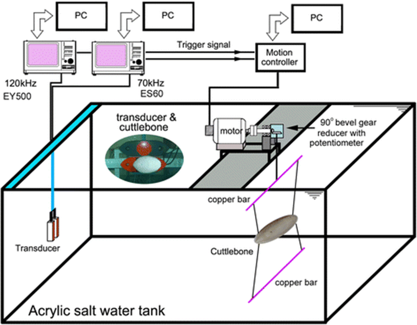
Before and near the end of the experiments, the 70 and 120 kHz echosounders were calibrated using copper spheres of 32.1 and 23.0 mm diameter, respectively. The TS measurements were corrected for these calibrated offsets (−0.3 dB at 70 kHz and 0.5 dB at 120 kHz).
The experiment was conducted under the guidelines of Animal Ethics Committee Regulations, No. 554 issued from Pukyong National University, Busan, Korea. Nineteen cuttlebones directly extracted from 19 of the 23 live cuttlefish individuals (with the exception of four broken cuttlebones) tested in our earlier study (Lee and Demer 2014) were used as specimens for the TS measurements. Each cuttlebone was carefully extracted from each live cuttlefish specimen in sea water just before the experiment, and then immediately moved to a small tank filled with seawater at 18 °C.
To avoid variations in the acoustic and physical properties of the extracted cuttlebone with time, especially due to changes in shape, structure, chamber space and density, the cuttlebone TS measurement was rapidly performed under almost identical conditions, but in another acrylic salt-water tank, following measurement of the TS of live cuttlefish.
Before each set of measurements, the specimen was carefully suspended into the overlapping sound beams, avoiding the introduction of air bubbles. The tilt angle of the cuttlebone was controlled using four monofilament lines (0.2 mm diameter), each tied to the anterior (head) and posterior (spine) parts of the cuttlebone, at both ends of an upper copper bar connected to the rotating axis of a DC servomotor system, and at both ends of a lower copper bar acting as a balancing weight (Fig. 1). The tilt angle was measured using a precision potentiometer (CP50, Sakae Tsushin Kogyo, Japan) connected to the axis of a 90° bevel gear reducer (ratio 240:1). The rotation speed of the cuttlebone was controlled by changing the input voltage of the DC servomotor system.
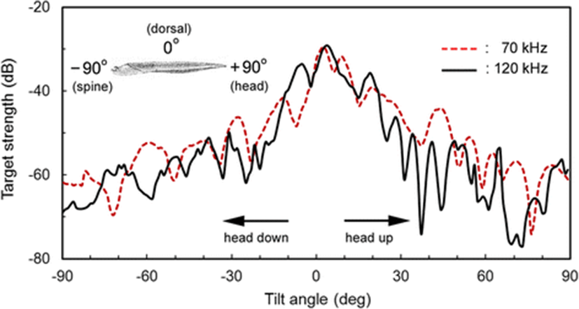
The definition of tilt angle for cuttlebone is shown in Fig. 2. The precise dorsal aspect of cuttlebone relative to the axis of the transducer was defined as a tilt angle of 0°, and the head up and down orientations relative to the center line of the cuttlebone were defined as positive θ and negative θ values, respectively.
In each case, the range between the transducers and the cuttlebone was approximately 1.2 m. The far-field ranges for the 70 and 120 kHz transducers (diameter d =13.5 and 12.9 cm) were ~0.47 and ~0.68 m (Lee 2006; Foote 2012), respectively. During the calibrations and the TS measurements, the 70 and 120 kHz echosounders transmitted 300 and 60 W pulses with durations of 256 μs and 300 μs every 0.2 s, and received the echoes using 6.2 and 12 kHz receiver bandwidths, respectively. The experiments in all cases were conducted using the same pulse duration, transmit power, pulse repetition interval and bandwidth used during the TS measurement of the calibration sphere. To avoid crosstalk, the measurements at 70 and 120 kHz were taken sequentially. When the trigger pulse of the echosounder was transferred to a PC-based motor controller (Comi-SD501, Comizoa, Korea) and signal processor (Comi-LX102, Comizoa, Korea), the TS measurement for the cuttlebone rotating at a fixed speed of 0.167 rpm, from the head-down orientation (−90°) to the head-up orientation (+90°), was conducted continuously. The output voltage of the precision potentiometer corresponding to the tilt angle and the echo data were recorded simultaneously and later processed to estimate the relationship between TS and tilt angle (θ) during each transmission. The echo data, logged by the echosounders, were post-processed using commercial software (Echoview V3.3, Sonar Data, Australia; EP500 v. 5.2, Simrad, Norway).
The biological and morphological characteristics of 19 specimens of cuttlebone and the corresponding live cuttlefish (Lee and Demer 2014) used in the TS experiments are shown in Table 1. These characteristics—such as length, weight, width and thickness—were measured following completion of the acoustic experiments. Mantle length (Lc) and body mass (Wc) for cuttlefish ranged from 156 to 203 mm (mean Lc = 173.9; deviation (std) = 13.10 mm) and 335–720 g (mean Wc = 527.4; std = 104.4 g), respectively. The length (Lb), weight (Wb), width (Wd) and thickness (Th) of cuttlebone ranged from 151 to 195 mm (mean Lb = 168.3; std = 12.56 mm), 29.3–53.2 g (mean Wb = 38.8; std = 7.23 g), 55–69 mm (mean Wd = 62.4; std = 4.10 mm), and 13.6–18.0 mm (mean Th = 15.7; std = 1.24 mm), respectively.
a The length of cuttlefish is a dorsal mantle length
The mean tilt angles (<θ>) with standard deviations (Sθ) measured for 19 live cuttlefish at 70 and 120 kHz in our earlier study (Lee and Demer 2014) are shown in Table 2. The TS and θ for these live cuttlefish were measured simultaneously using a split-beam echo sounder and a CCTV camera system, respectively and the (<θ>) and Sθ values were used in estimating the tilt-averaged TS from the TS functions of the corresponding cuttlebone.
In the 70 kHz experiments, the mean tilt angles of 19 live cuttlefish varied from −3.51° to −1.05° (mean −2.31°, head-down), while the standard deviation varied from 2.32° to 12.64° (mean 6.56°). At 120 kHz, the mean tilt angles varied from −5.11° to −0.73° (mean −3.15°), while the standard deviation varied from 2.33° to 6.86° (mean 4.74°).
To compare the TS of cuttlebone with that of live cuttlefish, two TS values, such as the maximum TS (TSm) and the tilt-averaged TS (<TSb>) in the dorsal-aspect orientation of the cuttlebone, were estimated. First, the TSm was obtained directly from the measured TS functions. Next, the < TSb > was calculated by using the probability density function f(θ) of tilt angle θ, with mean θ (<θ>) and standard deviation Sθ, according to Eqs. (1) and (2) (Foote 1980a, 1980b; Pena and Foote 2008):
where θ is the tilt angle defined as the angle made by the cuttlebone centerline with the horizontal, σ(θ) is the backscattering cross section of tilt angle θ and the tilt-angle distribution f(θ) was assumed to be a truncated normal distribution function. For each cuttlebone, the < TSb > was computed over the range < θ > −3 Sθ to < θ > +3 Sθ using the mean tilt angle (<θ>) with standard deviation (Sθ) indicated in Table 2.
Each dataset of the mean TS of cuttlebone and cuttlefish obtained for 19 specimens at 70 and 120 kHz was regressed on specimen length L and wavelength λ according to the empirical equation. First, to establish empirical single-frequency relationships between the < TS > and the corresponding L, the dataset for each frequency was independently fit, in the least-squares sense, to (Benoit-Bird et al. 2008; Conti and Demer. 2003; Demer and Martin 1995; Foote 1987; Goddard and Welsby 1986; Imaizumi et al. 2008; Kang et al. 2005; Sawada et al. 2011):
where L is the specimen length (cm), m is the slope of the regression line, and b is the intercept of the regression line on the TS axis.
Next, the datasets from both frequencies were combined to obtain a relationship for a wider range of specimen lengths (L) and wavelengths (λ):
where L is the specimen length (m), λ is the acoustic wavelength (m), and a, b, c are the fitted coefficients (Love 1969, 1971; McClatchie et al. 1996, 2003).
The mean TS (<TSc>) of live cuttlefish was derived from the results of TS measurements of the same specimen listed in Table 1 and described fully in our earlier study (Lee and Demer 2014). The influence of cuttlebone on the cuttlefish TS (<TSc>) was analyzed by estimating the difference between these mean TS values and by comparing the TS-length relationships for the corresponding cuttlebone and the cuttlefish at 70 and 120 kHz.
Results
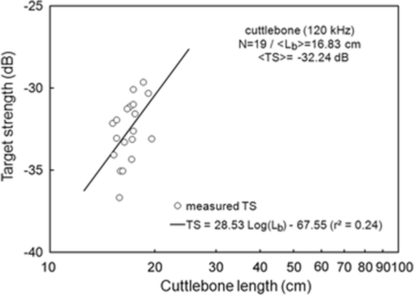
The < TSb > of 19 cuttlebones were plotted separately for 70 and 120 kHz versus cuttlebone length Lb, overlaid on the regressions of Eq. (3) (Figs. 3 and 4).
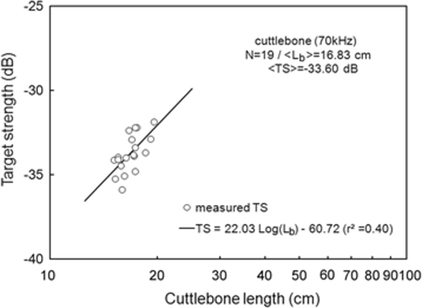
At 70 kHz,
At 120 kHz,
The mean < TSb > at 70 kHz was −33.60 dB, 1.36 dB lower than that at 120 kHz (−32.24 dB). The mean < TSb > at 70 kHz was 0.30 dB higher than that indicated by Eq. (5) and the mean < TSb > at 120 kHz was 0.33 dB higher than that indicated by Eq. (6). The difference between the slopes of the regressions for these frequencies was 6.5, and the intercept at 70 kHz was 6.83 dB higher than that at 120 kHz (Eqs. 5 and 6).
For 70 and 120 kHz combined, the 38 measurements of < TSb > and TSm were transformed to mean scattering cross-sectional areas (σ; m2) and σ2/λ was plotted versus L/λ (Fig. 5). In Fig. 5, the TSm in the dorsal-aspect orientation of cuttlebone was derived by simple extraction from the TS function measured as a function of tilt angle. The mean TS (<TSc>) of live cuttlefish was obtained from the results of TS measurements of the specimens listed in Table 1 and described fully in our earlier study (Lee and Demer 2014).
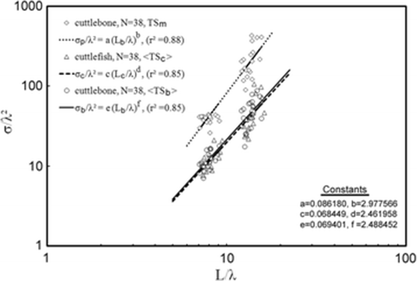
In this wavelength-normalized form, the TSm, <TSb>, and < TSc > values of cuttlebone are comparable between frequencies:
for TSm,for < TSb>, andfor < TSc>, where σp, σb, and σc are scattering cross-sectional areas (m2) corresponding to the TSm and < TSb > of cuttlebone and the < TSc > of cuttlefish, respectively.Using Eq. (4), the predicted TS’s of an individual specimen of cuttlebone and cuttlefish are indicated by:
for the predicted value (TSp) of TSm,for the predicted value (TSb) of < TSb>, andfor the predicted value (TSc) of < TSc>, where Lb and Lc are the length of cuttlebone (m) and the mantle length of cuttlefish (m), respectively and λ is the wavelength (m).The mean TSm values were −28.45 dB at 70 kHz and −25.59 dB at 120 kHz, respectively. These mean TSm values were 0.09 dB at 70 kHz and 0.71 dB at 120 kHz higher than those predicted by Eq. (10). The mean < TSb > values were −33.60 dB at 70 kHz and −32.24 dB at 120 kHz. These mean < TSb > values were 0.11 dB at 70 kHz and 0.33 dB at 120 kHz higher than those predicted by Eq. (11). The differences between the mean TSm and the mean < TSb > were 5.14 dB at 70 kHz and 6.65 dB at 120 kHz. The mean < TSc > values were −33.41 dB at 70 kHz and −32.20 dB at 120 kHz. These mean < TSc > values were 0.23 dB at 70 kHz and 0.35 dB at 120 kHz higher than that predicted by Eq. (12). Furthermore, for 70 and 120 kHz combined, the mean < TSc > value was −32.86 dB, 0.11 dB higher than the mean < TSb > value (−32.87 dB). On the other hand, the mean < TSc > predicted by Eq. (12) was −33.06 dB, 0.04 dB higher than the mean < TSb > predicted by Eq. (11) (−33.10 dB).
Accordingly, the contribution of cuttlebone to cuttlefish TS determined by the predicted results was slightly larger than that by the measured results. These results suggest that the cuttlebone is fully responsible for the TS of cuttlefish and the contribution is estimated to be more than 99 % of the total echo strength.
Discussion
An example of the 70 and 120 kHz echograms recorded as a function of tilt angle, as the cuttlebone is rotated from the spine-on aspect (−90°) toward the broadside incidence of the dorsal surface in the pitch plane, is shown in Fig. 5. At spine-on and head-on aspects, there was very weak scattering, and as the cuttlebone was approached from the spine-on aspect toward the broadside orientation, the scattering gradually increased. These angular and frequency dependences of acoustic scattering may allow the cuttlefish to be distinguishable from other fish species, which may be expected to have different responses at these frequencies. In particular, the angular dependence on the backscattering in the dorsal plane of the cuttlebone must be accounted for in relation to the improvement of the fish-sizing accuracy of split-beam echo sounders operating at these frequencies. It is also important to note that the tilt-angle dependence of the echo response in Fig. 6 is extremely complex due to the constructive and destructive interference effects of the backscattering signals generated by internal cuttlebone chambers.
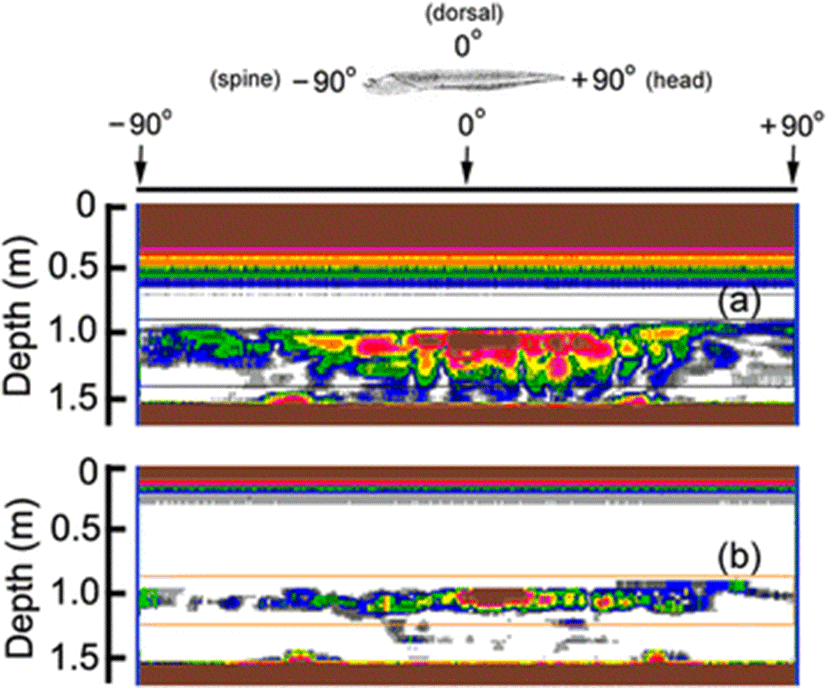
In our previous study (Lee and Demer 2014), the orientation for freely swimming cuttlefish was slightly angled head-down relative to the medial axis of the cuttlefish. The strongest backscattering in Fig. 6 was predicted to occur when the cuttlebone surface closest to the sound source is orthogonal to the transducer. However, because of the complexity of the chamber structure, density and curvature of the dorsal surface, the strong echo amplitudes in the echograms for 70 and 120 kHz occurred at slightly head-up aspects (positive tilt-angles).
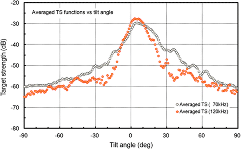
The measured TS functions, interpolated at 1° intervals, for 70 and 120 kHz are shown in Figs. 7 and 8, respectively; the tilt-averaged TS functions for all 19 cuttlebones were overlaid on the plot. In Figs. 7 and 8, a positive tilt angle indicates a head-up posture and a negative tilt angle indicates a head-down posture. The strongest responses were observed at slightly head-up aspects between 1° and 14° at 70 kHz and between 2° and 10° at 120 kHz, and weak responses of approximately −60 dB were observed near the spine-on (−90° aspect) and head-on (+90° aspect) orientations.
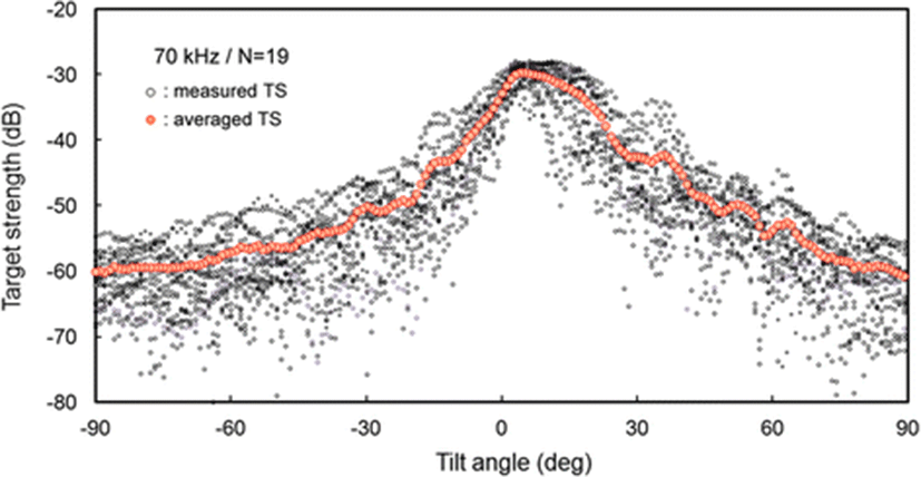
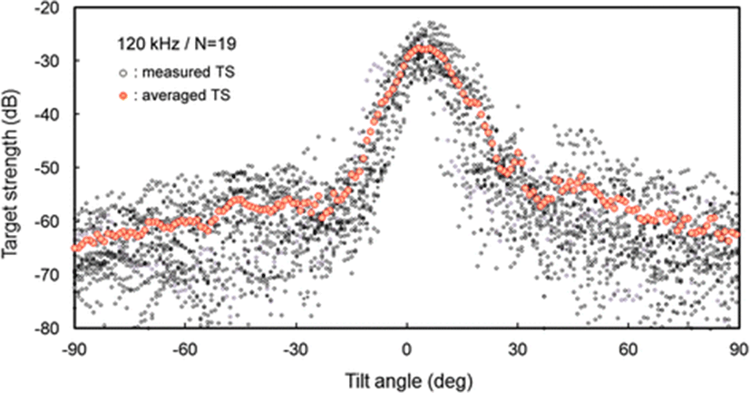
For each cuttlebone, these measured TS functions were used to calculate the mean TS over the range [<θ > −3 Sθ, <θ > +3 Sθ] from head-down to head-up orientations by Foote’s method (Foote 1980a, 1980b; Pena and Foote 2008). A comparison of the tilt-averaged TS functions of cuttlebone at 70 and 120 kHz is shown in Fig. 9. The tilt-averaged TS function for 120 kHz showed a strong directivity pattern with higher, narrower peaks and deeper nulls than for 70 kHz, and these TS patterns were essentially unimodal with the dominant peaks at slightly positive aspects; the tails in the anterior and posterior orientations extended down to ~60 dB. It appeared that the tilt-averaged TS function for 120 kHz exhibited a wider pattern near the peak than at 70 kHz (Fig. 9), but the broadening was due to the overlapping of TS patterns with different tilt angles for the peak positions (Figs. 7 and 8). The peak TS values in the tilt-averaged TS functions were −29.6 dB at a tilt angle of +5° for 70 kHz and −27.5 dB at a tilt angle of +3° for 120 kHz, respectively and the peak TS at 120 kHz was 2.1 dB higher that at 70 kHz.
Cuttlebone is bilaterally symmetrical in shape and derived from the juxtaposition of four parts: the outer cone, inner cone, phragmocone and spine. The dorsal surface of cuttlebone is evenly convex in outline but the anterior, median and posterior parts have slightly different curvatures (Neige 2003). Due to these morphological characteristics of cuttlebone, the dependence on the orientation of the cuttlebone TS is sensitive to the incidence direction (Figs. 7 and 8).
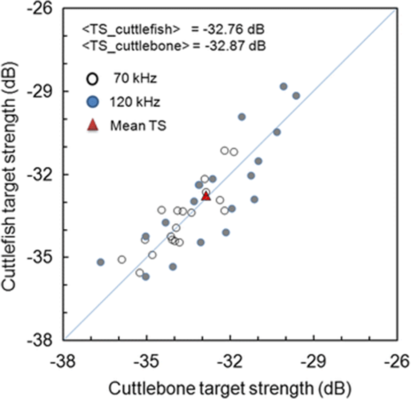
A comparison of the mean TS of cuttlefish with the mean TS of cuttlebone is shown in Fig. 10. A comparison of the measured and predicted contributions of cuttlebone to cuttlefish TS is shown in Table 3. In Table 3, the contributions are indicated as the differences between the mean TS values that are described within the 95 % confidence limits. In Fig. 10 and Table 3, the mean TS values measured using the combined dataset of all 38 specimens for 70 and 120 kHz were −32.76 dB for cuttlefish and −32.87 dB for cuttlebone; i.e., the mean TS of cuttlefish was 0.11 dB higher than that of cuttlebone. On the other hand, the mean TS values predicted by regressions of the combined dataset of all 38 specimens for 70 and 120 kHz were −33.06 dB for cuttlefish and −33.10 dB for cuttlebone; i.e., the mean TS of cuttlefish was 0.04 dB higher than that of cuttlebone. Accordingly, the contribution of cuttlebone to cuttlefish TS in the predicted results was slightly larger than in the measured results (Table 3). Furthermore, the measured mean TS values of cuttlefish and cuttlebone for a single frequency of 70 kHz were −33.41 and −33.60 dB, respectively; a 0.19 dB difference. The measured mean TS values of cuttlefish and cuttlebone at a single frequency of 120 kHz were −33.41 and −33.60 dB, respectively; a 0.19 dB difference. That is, the contribution of cuttlebone at 120 kHz was 0.15 dB higher than at 70 kHz (Table 3). On the other hand, the predicted mean TS values of cuttlefish and cuttlebone at a single frequency of 70 kHz were −33.63 and −33.71 dB, respectively; a 0.08 dB difference. The predicted mean TS values of cuttlefish and cuttlebone at a single frequency of 120 kHz were −32.55 and −32.60 dB, respectively, a 0.02 dB difference. That is, the contribution of cuttlebone at 120 kHz was 0.06 dB higher than at 70 kHz (Table 3).
The slopes of the regressions for a single frequency in this study were estimated to be 22.03 [95 % confidence interval (CI), 22.03 ± 13.87, P < 0.01] at 70 kHz and 28.53 [95 % CI, 28.53 ± 26.29, P < 0.05] at 120 kHz [Eqs. (5) and (6)]. These results suggest that the mean TS of cuttlebone varies with approximately the square power of the length at 70 and 120 kHz. The intercept [95 % CI, −60.72 ± 17.00 dB, P < 0.01] of the regression line at 70 kHz was 6.83 dB higher than at 120 kHz [95 % CI, −67.55 ± 32.21 dB, P < 0.01].
According to Simmonds and MacLennan (2005), the slope (m) and intercept (b) of cuttlefish vary widely versus fish species and commonly have values between 18 and 30 and 60 and 80, respectively. The slope and intercept in this study were within these ranges, although the determination coefficient (r2) indicated relatively low values of r2 = 0.40 at 70 kHz and r2 = 0.24 at 120 kHz. Compared to our earlier study (Lee and Demer 2014), the slopes for cuttlebone were 2.64 at 70 kHz and 12.06 at 120 kHz, lower than those of cuttlefish, and the intercepts for cuttlebone were 3.31 dB at 70 kHz and 15.41 dB at 120 kHz, higher than those of cuttlefish.
The chi-squared test of independence (CSTI, 99 % confidence level) for the TSm and the < TSb > values at 70 and 120 kHz showed that the TSm and the < TSb > values of cuttlebone at these two frequencies were independent (P > 0.01). Accordingly, to compare the TSm and the < TSb > values measured at multiple frequencies, a non-dimensional representation may be used (McClatchie et al. 1996; McClatchie et al. 2003, this study). In this study, the 38 wavelength-normalized TSm and < TSb > values measured at two frequencies from 19 cuttlebones were compared and showed length-dependent scattering [e.g., Eqs. (10), (11) and (12)]. This formulation allowed twice the number of measurements (38 vs. 19) to be combined in the regression (Love 1969, 1971), which resulted in a considerably better fit [r2 = 0.88 in Eq. (10), r2 = 0.85 in Eq. (11), and r2 = 0.85 in Eq. (12)] (Fig. 5). The fitted coefficient a, b and c values for the regressions of Eqs. (4) and (11) were 24.86 [95 % CI, 24.86 ± 3.57, P < 0.01], −4.86 [95 % CI, −4.86 ± 3.57, P < 0.01], and −22.58 [95 % CI, −22.58 ± 3.64, P < 0.01], respectively. In Fig. 5, the regression of the maximum TS (TSm), which is within the 95 % confidence limit, was ~5 dB higher than that of mean TS (<TSb>). Furthermore, at both frequencies, the contributions of the measured results were similar to those of the predicted results (Table 3). It is important to note that if the truncated limit of the tilt-angle distribution in the averaging operation by Foote’s method (Foote 1980a, 1980b; Pena and Foote 2008) is controlled, the contribution may be altered to some extent.
The TS of cuttlefish is expected to be markedly less depth-dependent than that of swimbladder fish because the buoyancy mechanism of cuttlebone, unlike the fish swimbladder, is almost independent of depth during vertical movements (Denton and Gilpin-Brown 1961; Denton et al. 1961; Denton and Taylor 1964). Knudsen and Gjelland (2004) reported that at least some coregonid species are capable of filling the swimbladder without access to the surface during the diel vertical migration and that TS did not decrease with depth. This swimbladder volume compensation in coregonids is compared to buoyancy regulation by the cuttlebone in cuttlefish. Generally, the change in the surface area of the swimbladder caused by the change in swimbladder volume affects TS, but because the dorsal surface of cuttlebone is unaffected by depth, the depth effect of cuttlebone on cuttlefish TS is not expected to be affected like the swimbladder of fish. Instead of having a flexible swimbladder like a fish, cuttlefish have a cuttlebone, which has a rigid structure, for buoyancy control. The cuttlebone is divided by many thin, chitinous partitions, which separate gas-filled anterior chambers and fluid-filled posterior chambers of approximately periodic microstructure (Denton and Gilpin-Brown 1961; Denton et al. 1961; Denton and Taylor 1964; Neige 2003; Cadman et al. 2010a, 2010b; Chen et al.2011). Unlike the swim bladder of fish, cuttlebone is unpressurized, so its volume is not altered markedly as the animal changes depth (Denton and Gilpin-Brown 1961; Denton et al. 1961; Denton and Taylor 1964), and no adjustments to the buoyancy system are necessary during vertical movements (Sherrard 2000).
Generally, the fish TS is proportional to the difference in density between the insonified fish target and the surrounding water (Simmonds and MacLennan 2005), and the main source of backscatter is expected to be proportional to the size of the swimbladder, which accounts for at least 90 % of echo energy (Foote 1980a, 1980b, 1985; Foote and Ona 1985). The impedance of gas-filled organs, such as the swimbladder and cuttlebone, differs considerably from that of seawater and other fish tissues, and the scattering contribution of cuttlebone is comparable to that of an air-filled swimbladder. However, in cuttlefish, the problems of pressure changes are avoided by enclosing the gas in the cuttlebone, the volume of which is unaffected by changes in depth and which contains many chambers, some filled with gas and some with liquid. The overall density of the cuttlebone varies between ~0.5 and 0.7, and is controlled by regulating its liquid content (Denton and Gilpin-Brown 1961; Denton et al. 1961; Denton and Taylor 1964). Accordingly, the acoustic scattering by cuttlefish is expected to fluctuate in proportion with changes in the overall density of cuttlebone. Madsen et al. (2007) reported that the muscular mantle and fins of the common squid are the dominant scatterers, and that the hard parts—such as beak, eyes and pen—contribute little to the TS of squid, at least for frequencies representative of the clicks of most teutophageous toothed whales. This suggests that the acoustic interference of the muscular mantle, fins and cuttlebone in freely swimming cuttlefish are complexly generated based on frequency.
In this study, the TS of cuttlebone was measured and analyzed as a function of length only; however, the TS may actually be more sensitive to the dorsal surface area (or volume) of cuttlebone rather than the length. Based on a comparison of the TS-L relationships for the corresponding cuttlebone and live cuttlefish for 19 specimens, the contribution of cuttlebone to the backscattering echo strength of cuttlefish was estimated to be at least 99 %. Moreover, the cuttlebone volume (or surface area) may have a greater influence on cuttlefish TS than the length, because the proportion of cuttlebone volume as a fraction of the total body volume of cuttlefish (~9.3 %) is almost twofold that of the swimbladder of fish (~5 %) (Denton and Gilpin-Brown 1961; Denton et al. 1961; Denton and Taylor 1964). The relationship between cuttlebone volume and cuttlefish TS may be complicated by the complex microstructure of the gas-filled internal shell of the cuttlebone. However, the effects of the morphological and material parameters of cuttlebone—such as length, width, height, density change and curvature of the dorsal surface—must be analyzed to quantitatively estimate the influence of cuttlebone on cuttlefish TS. This will be the subject of a future study.
Conclusions
The mean TS values of cuttlebone were 0.19 and 0.04 dB lower than those of cuttlefish at 70 and 120 kHz, respectively. The contribution of cuttlebone to the cuttlefish TS determined by the measured results was slightly greater than that by the predicted results. From these results, we concluded that cuttlebone is responsible for the TS of cuttlefish, and the contribution is estimated to be at least 99 % of the total echo strength.